Four Years Remaining

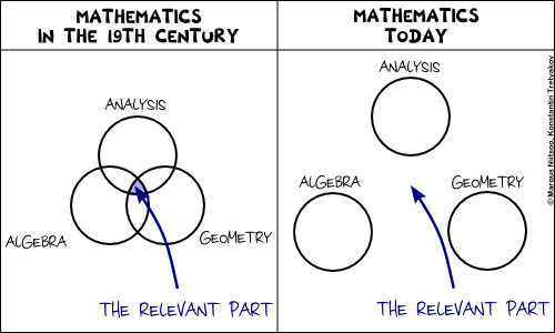
A cute joke by Margus from the recent EWSCS09 Crapcon session.

Symbols and Reality

Mathematics is a language. An abstract set of generic symbols for describing concepts, objects and systems. Take, for example, the symbol "5", "five". What is it? Is it a real-world object? No. It is just a symbol. You are free to attach to it any interpretation that you deem appropriate. Of course, most of the times you would use the common interpretation of "5" as a natural number, denoting, well, "five of something". Literally meaning that you can count something as "this, this, this, this and this".

Take a moment to reflect on the degree of generality of this simple concept, "five". It can be applied to practically anything. Five apples, five centimeters, five centuries are notions as different from each other as you could imagine, and yet all of them relate to the concept "five". On the other hand, it is not too generic to be useless: "five" is radically different from "six", "seven", and an infinity of other numbers. This kind of magical balance between generality and specificity is common to mathematics. This is what makes mathematics both widely applicable and yet still incredibly useful.

Besides just giving us symbols like 5 or 6, mathematics provides an endless variety of ways for expressing "rules", "operations", "statements", "derivations", "computations" and the like, such as 5+5=10, or , etc. Once again, all of these rules, operations and statements need not necessarily bear any relation with reality. After all, they all are just a cunning play with symbols. And yet, quite often they do describe reality incredibly well. I know that 512 apples and 512 apples will make 1024 apples together. How do I know it? Certainly not because I checked it on real apples! I just believe that the real-world operation of "adding apples" can be satisfactory modeled using the formal symbolic framework of natural numbers and the operation of addition on them. Why do I believe it? This is a tricky philosophical question that we shall leave aside for now. But remember that any application of mathematics to the real world is always based on a belief that the chosen model describes the world well.

The Nature of Uncertainty

There are often cases where we would like to use mathematics to model "uncertainty". Now remember that from the point of view of pure math there are no such things as inherent "certainty" and "uncertainty". Mathematics will always operate on symbols and use precise, uniquely reproducible transformation rules between these symbols. Yet there are often cases when we, in our interpretations of these symbols, would like refer to certain entities as "uncertain". The reasons can be various:

1. Sometimes, we would like to use a single generalized concept to summarize multiple objects.
   - What is the height of a human?
   There is no single clear answer and yet it is possible to provide one using an uncertainty model such as a probability distribution.
2. Sometimes, we want to reason about some single numeric value which, even if it were well-defined, we just could not compute exactly.
   - What is the AVERAGE height of a human?
   In theory, it is a number you could measure by lining up all the people in the world and computing their average, but it is certainly an infeasible project.
3. Sometimes, the notion we would like to reason about is inherently not well-defined.
   - What is MY height, after all?
   The answer depends on a number of factors such as time, measuring equipment, my precise posture, etc. Instead of taking all of these into consideration, we prefer to exploit an uncertainty model.
4. Sometimes we just need a single concept to encapsulate a state of knowledge more sophisticated than pure numeric equality. For example, to express the fact like "my height IS GREATER THAN 150cm" without using the "greater than" operation.

There are also other situations, which are difficult to classify, but in all cases the idea is the same — for one reason or another we "don't know" (or "don't specify") the exact single quantity we want to reason about, an yet we still "know something" about it. In fact, amusingly, the amount of information that we use to represent an "uncertain" quantity is often much greater than the amount of information we would need to represent a "certain" one. For example, there are much more probability distributions than there are real numbers. Therefore, picking one probability distribution to represent our knowledge of a number is, in principle, a more informative step than picking a single real number. And yet, we call the former case "uncertainty" and the latter one "certainty". Because that's how we choose to name and interpret things, that's how we believe these concepts relate to reality.

Models of Uncertainty

The adjective "uncertain" is something you could, in theory, apply generically to any type of data. In a computer scientist's terms, it makes perfect sense to talk about datatypes "uncertain int", "uncertain real", "uncertain boolean", "uncertain string", "uncertain graph", "uncertain map" and maybe even "uncertain uncertain real" and the like. Let's limit ourselves here to the consideration of uncertain numbers only, as these are the most commonly used and well-studied types of uncertainty. So how do you model (or, say, "implement") "uncertain real"? Here is a short list of the most popular options:

1. Approximate numbers.Although you might not consider it as a smart approach, this is probably the most common choice in practice — using a usual number to represent an uncertain one. In this case the uncertainty is purely interpretative: instead of stating you would, perhaps, write , denoting your state of ignorance. Quite often you would not even care to use the approximate equality sign, presuming it is clear from the context that you are not supposed to provide an ideally exact measurement: — What is your height? — It is 180cm. This works quite well in simple real-life situations, such as buying a kilogram of apples or discussing the horsepowers in a friend's motorbike, but is also applicable to some more technical cases, such as computing the distance to the nearest star.The advantage of such implied uncertainty is that you do not really need to deal with it. All of your familiar arithmetic operations come for free, together with their well established interpretations and the nice properties, theories and theorems. The disadvantage is that once your data is approximate, all of these theories and theorems become approximate too. So, although it could often be acceptable to claim , you would have problems explaining more complicated steps, such as " for a continuous f".But what to do if you need to perform such steps? Consider intervals instead!
2. Intervals.The second most popular method of representing an uncertain real number is to provide an interval where it falls into. It is ubiquitous in engineering disciplines. Most often an interval is expressed either as or by following the significant figures convention (e.g. writing 180.00 to denote 180±0.01). It is an improvement over the previous approach, because now you have a way to quantify the effect of function application on uncertainty. For example, a commonly used rule would be

   ,

   where f is a differentiable function.

3. Sets.An approach slightly more general than the "interval" technique would be to provide a set of values, to which the value of interest could belong to. So, instead of stating x = 5 you could write, for example, .This allows for more mathematical rigour. For example: . Moreover, besides the standard algebraic operations, the set representation allows to update the knowledge about an uncertain value easily using set unions and intersections:

   .

   However, sets are "heavy" object to work with, so you don't see this approach being used too often in practical computations. Some Monte-Carlo simulations would use a set to represent approximate solutions, but they would convert it to a probability distribution as soon as possible. This leads us to the next item on the list.

4. Probability distributions.If the previous methods were either too crude, too ad-hoc or too heavy, then probability theory was designed to provide flexible balance and help overcome most of their drawbacks. To represent a number it suggests us to use a probability measure - an additive function that assigns a weight to each set, which could contain the value of interest. The greater the weight of a set - the more probable it is that the value belongs to that set. By convention, the minimum possible weight of a set is 0, which we usually interpret as "the value almost certainly does not belong to that set", and the maximum weight is 1, with a corresponding interpretation "the value almost certainly belongs there". Representing a function defined on sets is complicated, so usually we use a simpler equivalent representation: a cumulative distribution function (CDF) or a probability density function (PDF). The plot of the latter is especially insightful and provides a nice visual cue about the nature of uncertainty being modeled.It is impossible to enumerate all the virtues of using a probability distribution as an uncertainty model. A probability distribution is a flexible structure, capable of accomodating most "common" kinds of uncertainty. There is an authoritative, well-developed theory and a wide range of both practical and theoretical tools available. Besides the standard algebraic operations, you have rules for updating knowledge (such as the Bayes rule) and a range of facilities for decision making (estimation, hypothesis testing, etc). Finally, there are various interpretations available for you to choose from.Of course, there are potential drawbacks, too. On the practical side, it is not always computationally convenient to work with a probability measure. It is a function, after all, and when specified arbitrarily it can either take too much space to represent or too much time to compute. The use of smoothing and approximation techniques can somewhat relieve the problem, but comes at the price of additional assumptions and simplifications. Secondly, a probability distribution is not capable of representing any kind of uncertainty: for example, there is no probability distribution corresponding to the statement "x < 5". Thirdly, the requirement for a probability density to be normalized to sum to 1 is sometimes inconvenient (because you have to normalize) or unintuitive (because it seems to declare that there is a single uncertain value "hidden inside").

   

   For example, consider the picture on the right and try to provide a concise description of the set of black pixels on it. This will be an uncertain notion because, well, a gray pixel is also somewhat black, isn't it? And although you could provide a probability distribution of "black" on the picture, you would probably intuitively prefer to assign a "truth-value" between 0 and 1 to each pixel, with 1 corresponding to "certainly black" and 0 to "certainly not black". This would, however, violate the "sum-to-one" normalization rule and thus would not be a probability density. What would it be? A fuzzy set.

5. Fuzzy sets.A fuzzy set is a set whose elements can have a degree of membership between 0 and 1. It is therefore something inbetween a set (because it "feels" like a set) and a probability density (because it is a function, only this time normalized to have a maximum of 1, instead of the integral of 1). A person familiar with probability theory will also easily recognize a straightforward analogy of a fuzzy set to a likelihood function.Fuzzy sets seem to be a natural uncertainty model in various circumstances, such as the "black pixels" example above. They are often conceptually simpler to specify than probability densities, and lack the interpretation controversy surrounding probability theory. On the other hand, the theory of fuzzy sets is not as extensive as that of probabilities. It is rich in operations like max and min, which makes some things computationally difficult. Besides, the lack of a universal interpretation for fuzzy membership values results in a lack of simple unique decision-making facilities. There are just way too many defuzzification rules to choose from.
6. ... and more.A variety of other approaches is available, the most important ones being Possibility theory, and Dempster-Shafer theory. However, as this text has already grown too long for a blog post, I shall leave the detailed description of these to Wikipedia.

Summary

The main message of this exposition is actually quite simple. There are various approaches to modeling uncertainty. They differ in the type of supported operations and, most importantly, in the way we interpret them and map to the real world entities. But nonetheless, these are all still just methods for modeling uncertainty, each with its own advantages and limitations. Moreover, in most situations, as long as you use the math "reasonably", the models are approximately equivalent in terms of the results and decisions you might end up with using them. That is probably the reason why practitioners would rarely consider anything more sophisticated than a probability measure (except, perhaps, when they are feeling adventurous). And that is why it can sometimes be complicated to promote the more "modern" approaches without the awkward looks from the side of the "traditional statistics". After all, these approaches are competing on the same field with The One and Only, Probability Theory.

The yachts parked in the port of Palma de Mallorca might very well outnumber the presumably plentiful palm trees in this city. The photo below depicts just a small piece of the 3 kilometer-long marina, stretched along the Paseo Maritimo coastline.

Yachts in Palma de Mallorca

For the fun of it, let's try counting the yachts on this photo. Even though it is perhaps one of the most useless exercises one might come up with, I find it amusing and not without a relation to a variety of more serious applications. Naturally, no sane computer scientist would attempt to do the counting manually when he can let a computer do this job for him. Therefore, we'll use a chance here to exploit the fantastic Scilab Image Processing toolbox.

Preprocessing

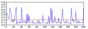
If we only want to know the number of masts, we don't need the whole image, a single line of the image that crosses all of the masts would suffice. Some pixels of this line will correspond to the sky — a brief examination shows that the RGB colour of these pixels is approximately (0.78, 0.78, 0.78). The remaining pixels will be the masts and the ropes. For each pixel, we can compute how similar this pixel's colour is to the colour of the sky (the simple euclidean distance will do OK), and thus we shall end up with a single vector, the peaks in which will correspond to the masts we need to count.

  // Read image
  img = imread("yachts.jpg");

  // Get the proper line
  img_line = img(505,:,:);

  // Subtract sky colour
  img_line = sqrt(sum((img_line - 0.78*ones(img_line)).^2, 3));

The vector to be analyzed (its first 200 pixels out of 1600 total)

Let us now do the counting.

1. Geometric approach

A look on the picture above will tell you that a threshold of about 0.2 might be good for discriminating the masts from the background. Once we apply it, there are at least two easy ways to derive the number of masts.

• Firstly, we could count the number of pixels over the threshold and divide it by four, which seems like roughly the average width of a mast.

     answer = sum(img_line > 0.2)/4

  The result is ~135.

• Secondly, we could count the number of times the pixel value crosses the 0.2 boundary:

     answer = sum(img_line(2:$) > 0.2  & img_line(1:($-1)) <= 0.2);

  Here the result will be 158.

2. Spectral approach

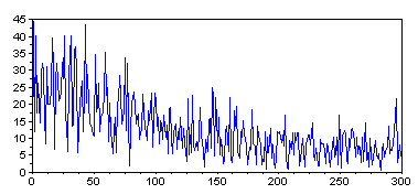
The discrete Fourier transform of a vector is a natural way for counting repeating peaks in the signal.

  ff = abs(fft(center(img_line)));
  plot(0:300, ff(1:301));

Masts vector spectrum

The interpretation of the resulting figure should, in theory, be simple. If the photo only contained n uniformly distributed masts, the spectrum would have one clear peak at n. In our case, unfortunately, things do not seem to be as easy. With some wishful thinking one might see major peaks around 50, 150 and 300. Now taking the previous results into consideration let us presume that 150 is the correct peak. Then 50 could correspond to the 50 "larger" masts on the image, and 300, perhaps, to the ropes.

3. Statistical approach

The original image is 1600 pixels wide. If the photo contained n masts, distributed uniformly along its width, a randomly chosen 32-pixel region would contain about n/50 masts on average. Therefore, let us select some of these random regions and count the number of masts in them manually. After multiplying the resulting numbers by 50 we should obtain estimates of the total number of masts.

  xbasc();
  rand("seed", 1);
  for i=1:9
    m = floor(rand()*(1600-32))+1;
    subplot(3,3,i);
    imshow(img([474:566], [m:(m+32)],:))
  end

Here are the estimates I got here: 200, 50, 50, 150, 150, 100, 100, 100, 100. The average comes at 111 with a standard deviation of about 50.

Summary

There are serious discrepances among the results produced by various approaches. However, if you attempt to count the masts manually, you will quickly discover that there is indeed an inherent degree of uncertainty in the number of visible masts, with the true number lying somewhere between 100 and 150. Consequently, the considered approaches to mast counting were not too far off, after all.