By popular suggestion this text was cross-posted to Medium.
Suppose you are starting a new data science project (which could either be a short analysis of one dataset, or a complex multi-year collaboration). How should your organize your workflow? Where do you put your data and code? What tools do you use and why? In general, what should you think about before diving head first into your data? In the software engineering industry such questions have some commonly known answers. Although every software company might have its unique traits and quirks, the core processes in most of them are based on the same established principles, practices and tools. These principles are described in textbooks and taught in universities.
Data science is a less mature industry, and things are different. Although you can find a variety of template projects, articles, blogposts, discussions, or specialized platforms (open-source [1,2,3,4,5,6,7,8,9,10], commercial [11,12,13,14,15,16,17] and in-house [18,19,20]) to help you organize various parts of your workflow, there is no textbook yet to provide universally accepted answers. Every data scientist eventually develops their personal preferences, mostly learned from experience and mistakes. I am no exception. Over time I have developed my understanding of what is a typical "data science project", how it should be structured, what tools to use, and what should be taken into account. I would like to share my vision in this post.
The workflow
Although data science projects can range widely in terms of their aims, scale, and technologies used, at a certain level of abstraction most of them could be implemented as the following workflow:
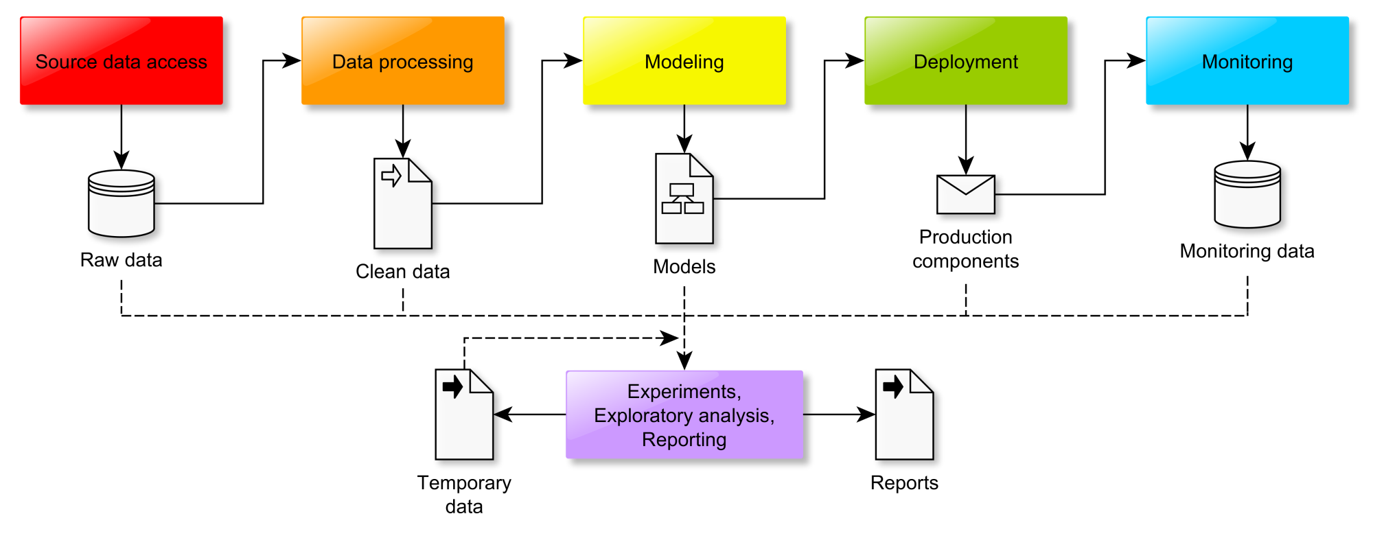
Colored boxes denote the key processes while icons are the respective inputs and outputs. Depending on the project, the focus may be on one process or another. Some of them may be rather complex while others trivial or missing. For example, scientific data analysis projects would often lack the "Deployment" and "Monitoring" components. Let us now consider each step one by one.
Source data access
Whether you are working on the human genome or playing with iris.csv, you typically have some notion of "raw source data" you start your project with. It may be a directory of *.csv files, a table in an SQL server or a HDFS cluster. The data may be fixed, constantly changing, automatically generated or streamed. It could be stored locally or in the cloud. In any case, your first step is to define access to the source data. Here are some examples of how this may look like:
- Your source data is provided as a set of
*.csvfiles. You follow the cookiecutter-data-science approach, make adata/rawsubdirectory in your project's root folder, and put all the files there. You create thedocs/data.rstfile, where you describe the meaning of your source data. (Note: Cookiecutter-DataScience template actually recommendsreferences/as the place for data dictionaries, while I pesonally preferdocs. Not that it matters much). - Your source data is provided as a set of
*.csvfiles. You set up an SQL server, create a schema namedrawand import all your CSV files as separate tables. You create thedocs/data.rstfile, where you describe the meaning of your source data as well as the location and access procedures for the SQL server. - Your source data is a messy collection of genome sequence files, patient records, Excel files and Word documents, which may later grow in unpredicted ways. In addition, you know that you will need to query several external websites to receive extra information. You create an SQL database server in the cloud and import most of the tables from Excel files there. You create the
data/rawdirectory in your project, put all the huge genome sequence files into the dna subdirectory. Some of the Excel files were too dirty to be imported into a database table, so you store them indata/raw/unprocesseddirectory along with the Word files. You create an Amazon S3 bucket and push your wholedata/rawdirectory there using DVC. You create a Python package for querying the external websites. You create thedocs/data.rstfile, where you specify the location of the SQL server, the S3 bucket, the external websites, describe how to use DVC to download the data from S3 and the Python package to query the websites. You also describe, to the best of your understanding, the meaning and contents of all the Excel and Word files as well as the procedures to be taken when new data is added. - Your source data consists of constantly updated website logs. You set up the ELK stack and configure the website to stream all the new logs there. You create
docs/data.rst, where you describe the contents of the log records as well as the information needed to access and configure the ELK stack. - Your source data consists of 100'000 colored images of size 128x128. You put all the images together into a single tensor of size 100'000 x 128 x 128 x 3 and save it in an HDF5 file
images.h5. You create a Quilt data package and push it to your private Quilt repository. You create thedocs/data.rstfile, where you describe that in order to use the data it must first be pulled into the workspace viaquilt install mypkg/imagesand then imported in code viafrom quilt.data.mypkg import images. - Your source data is a simulated dataset. You implement the dataset generation as a Python class and document its use in a
README.txtfile.
In general, remember the following rules of thumb when setting up the source data:
- Whenever you can meaningfully store your source data in a conveniently queryable/indexable form (an SQL database, the ELK stack, an HDF5 file or a raster database), you should do it. Even if your source data is a single
csvand you are reluctant to set up a server, do yourself a favor and import it into an SQLite file, for example. If your data is nice and clean, it can be as simple as:import sqlalchemy as sa import pandas as pd e = sa.create_engine("sqlite:///raw_data.sqlite") pd.read_csv("raw_data.csv").to_sql("raw_data", e) - If you work in a team, make sure the data is easy to share. Use an NFS partition, an S3 bucket, a Git-LFS repository, a Quilt package, etc.
- Make sure your source data is always read-only and you have a backup copy.
- Take your time to document the meaning of all of your data as well as its location and access procedures.
- In general, take this step very seriously. Any mistake you make here, be it an invalid source file, a misunderstood feature name, or a misconfigured server may waste you a lot of time and effort down the road.
Data processing
The aim of the data processing step is to turn the source data into a "clean" form, suitable for use in the following modeling stage. This "clean" form is, in most cases, a table of features, hence the gist of "data processing" often boils down to various forms of feature engineering. The core requirements here are to ensure that the feature engineering logic is maintainable, the target datasets are reproducible and, sometimes, that the whole pipeline is traceable to the source representations (otherwise you would not be able to deploy the model). All these requirements can be satisfied, if the processing is organized in an explicitly described computation graph. There are different possibilities for implementing this graph, however. Here are some examples:
- You follow the cookiecutter-data-science route and use Makefiles to describe the computation graph. Each step is implemented in a script, which takes some data file as input and produces a new data file as output, which you store in the
data/interimordata/processedsubdirectories of your project. You enjoy easy parallel computation viamake -j <njobs>. - You rely on DVC rather than Makefiles to describe and execute the computation graph. The overall procedure is largely similar to the solution above, but you get some extra convenience features, such as easy sharing of the resulting files.
- You use Luigi, Airflow or any other dedicated workflow management system instead of Makefiles to describe and execute the computation graph. Among other things this would typically let you observe the progress of your computations on a fancy web-based dashboard, integrate with a computing cluster's job queue, or provide some other tool-specific benefits.
- All of your source data is stored in an SQL database as a set of tables. You implement all of the feature extraction logic in terms of SQL views. In addition, you use SQL views to describe the samples of objects. You can then use these feature- and sample-views to create the final modeling datasets using auto-generated queries like
select
   s.Key
   v1.AverageTimeSpent,
   v1.NumberOfClicks,
   v2.Country
   v3.Purchase as Target
from vw_TrainSample s
left join vw_BehaviourFeatures v1 on v1.Key = s.Key
left join vw_ProfileFeatures v2 on v2.Key = s.Key
left join vw_TargetFeatures v3 on v3.Key = s.Key
This particular approach is extremely versatile, so let me expand on it a bit. Firstly, it lets you keep track of all the currently defined features easily without having to store them in huge data tables - the feature definitions are only kept as code until you actually query them. Secondly, the deployment of models to production becomes rather straightforward - assuming the live database uses the same schema, you only need to copy the respective views. Moreover, you may even compile all the feature definitions into a single query along with the final model prediction computation using a sequence of CTE statements:
with _BehaviourFeatures as (
 ... inline the view definition ...
),
_ProfileFeatures as (
 ... inline the view definition ...
),
_ModelInputs as (
 ... concatenate the feature columns ...
)
select
     Key,
     1/(1.0 + exp(-1.2 + 2.1*Feature1 - 0.2*Feature3)) as Prob
from _ModelInputs
This technique has been implemented in one in-house data science workbench tool of my design (not publicly available so far, unfortunately) and provides a very streamlined workflow.
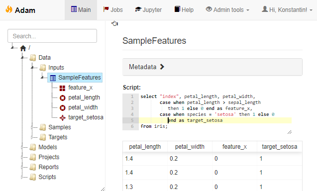
Example of an SQL-based feature engineering pipeline
No matter which way you choose, keep these points in mind:
- Always organize the processing in the form of a computation graph and keep reproducibility in mind.
- This is the place where you have to think about the compute infrastructure you may need. Do you plan to run long computations? Do you need to parallelize or rent a cluster? Would you benefit from a job queue with a management UI for tracking task execution?
- If you plan to deploy the models into production later on, make sure your system will support this use case out of the box. For example, if you are developing a model to be included in a Java Android app, yet you prefer to do your data science in Python, one possibility for avoiding a lot of hassle down the road would be to express all of your data processing in a specially designed DSL rather than free-from Python. This DSL may then be translated into Java or an intermediate format like PMML.
- Consider storing some metadata about your designed features or interim computations. This does not have to be complicated - you can save each feature column to a separate file, for example, or use Python function annotations to annotate each feature-generating function with a list of its outputs. If your project is long and involves several people designing features, having such a registry may end up quite useful.
Modeling
Once you have done cleaning your data, selecting appropriate samples and engineering useful features, you enter the realm of modeling. In some projects all of the modeling boils down to a single m.fit(X,y) command or a click of a button. In others it may involve weeks of iterations and experiments. Often you would start with modeling way back in the "feature engineering" stage, when you decide that outputs of one model make for great features themselves, so the actual boundary between this step and the previous one is vague. Both steps should be reproducible and must make part of your computation graph. Both revolve around computing, sometimes involving job queues or clusters. None the less, it still makes sense to consider the modeling step separately, because it tends to have a special need: experiment management. As before, let me explain what I mean by example.
- You are training models for classifying Irises in the
iris.csvdataset. You need to try out ten or so standardsklearnmodels, applying each with a number of different parameter values and testing different subsets of your handcrafted features. You do not have a proper computation graph or computing infrastructure set up - you just work in a single Jupyter notebook. You make sure, however, that the results of all training runs are saved in separate pickle files, which you can later analyze to select the best model. - You are designing a neural-network-based model for image classification. You use ModelDB (or an alternative experiment management tool, such as TensorBoard, Sacred, FGLab, Hyperdash, FloydHub, Comet.ML, DatMo, MLFlow, ...) to record the learning curves and the results of all the experiments in order to choose the best one later on.
- You implement your whole pipeline using Makefiles (or DVC, or a workflow engine). Model training is just one of the steps in the computation graph, which outputs a
model-<id>.pklfile, appends the model final AUC score to a CSV file and creates amodel-<id>.htmlreport, with a bunch of useful model performance charts for later evaluation. - This is how experiment management / model versioning looks in the UI of the custom workbench mentioned above:
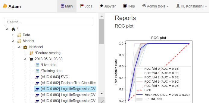
Experiment management
The takeaway message: decide on how you plan to manage fitting multiple models with different hyperparameters and then selecting the best result. You do not have to rely on complex tools - sometimes even a manually updated Excel sheet works well, when used consistently. If you plan lengthy neural network trainings, however, do consider using a web-based dashboard. All the cool kids do it.
Model deployment
Unless your project is purely exploratory, chances are you will need to deploy your final model to production. Depending on the circumstances this can turn out to be a rather painful step, but careful planning will alleviate the pain. Here are some examples:
- Your modeling pipeline spits out a pickle file with the trained model. All of your data access and feature engineering code was implemented as a set of Python functions. You need to deploy your model into a Python application. You create a Python package which includes the necessary function and the model pickle file as a file resource inside. You remember to test your code. The deployment procedure is a simple package installation followed by a run of integration tests.
- Your pipeline spits out a pickle file with the trained model. To deploy the model you create a REST service using Flask, package it as a docker container and serve via your company's Kubernetes cloud. Alternatively, you upload the saved model to an S3 bucket and serve it via Amazon Lambda. You make sure your deployment is tested.
- Your training pipeline produces a TensorFlow model. You use Tensorflow Serving (or any of the alternatives) to serve it as a REST service. You do not forget to create tests and run them every time you update the model.
- Your pipeline produces a PMML file. Your Java application can read it using the JPMML library. You make sure that your PMML exporter includes model validation tests in the PMML file.
- Your pipeline saves the model and the description of the preprocessing steps in a custom JSON format. To deploy it into your C# application you have developed a dedicated component which knows how to load and execute these JSON-encoded models. You make sure you have 100% test coverage of your model export code in Python, the model import code in C# and predictions of each new model you deploy.
- Your pipeline compiles the model into an SQL query using SKompiler. You hard-code this query into your application. You remember about testing.
- You train your models via a paid service, which also offers a way to publish them as REST (e.g. Azure ML Studio, YHat ScienceOps). You pay a lot of money, but you still test the deployment.
Summarizing this:
- There are many ways how a model can be deployed. Make sure you understand your circumstances and plan ahead. Will you need to deploy the model into a codebase written in a different language than the one you use to train it? If you decide to serve it via REST, what load does the service expect, should it be capable of predicting in batches? If you plan to buy a service, estimate how much it will cost you. If you decide to use PMML, make sure it can support your expected preprocessing logic and that fancy Random Forest implementation you plan to use. If you used third party data sources during training, think whether you will need to integrate with them in production and how will you encode this access information in the model exported from your pipeline.
- As soon as you deploy your model to production, it turns from an artefact of data science to actual code, and should therefore be subject to all the requirements of application code. This means testing. Ideally, your deployment pipeline should produce both the model package for deployment as well as everything needed to test this model (e.g. sample data). It is not uncommon for the model to stop working correctly after being transferred from its birthplace to a production environment. It may be be a bug in the export code, a mismatch in the version of
pickle, a wrong input conversion in the REST call. Unless you explicitly test the predictions of the deployed model for correctness, you risk running an invalid model without even knowing it. Everything would look fine, as it will keep predicting some values, just the wrong ones.
Model monitoring
Your data science project does not end when you deploy the model to production. The heat is still on. Maybe the distribution of inputs in your training set differs from the real life. Maybe this distribution drifts slowly and the model needs to be retrained or recalibrated. Maybe the system does not work as you expected it to. Maybe you are into A-B testing. In any case you should set up the infrastructure to continuously collect data about model performance and monitor it. This typically means setting up a visualization dashboard, hence the primary example would be the following:
- For every request to your model you save the inputs and the model's outputs to logstash or a database table (making sure you stay GDPR-compliant somehow). You set up Metabase (or Tableau, MyDBR, Grafana, etc) and create reports which visualize the performance and calibration metrics of your model.
Exploration and reporting
Throughout the life of the data science project you will constantly have to sidestep from the main modeling pipeline in order to explore the data, try out various hypotheses, produce charts or reports. These tasks differ from the main pipeline in two important aspects.
Firstly, most of them do not have to be reproducible. That is, you do not absolutely need to include them in the computation graph as you would with your data preprocessing and model fitting logic. You should always try to stick to reproducibility, of course - it is great when you have all the code to regenerate a given report from raw data, but there would still be many cases where this hassle is unnecessary. Sometimes making some plots manually in Jupyter and pasting them into a Powerpoint presentation serves the purpose just fine, no need to overengineer.
The second, actually problematic particularity of these "Exploration" tasks is that they tend to be somewhat disorganized and unpredictable. One day you might need to analyze a curious outlier in the performance monitoring logs. Next day you want to test a new algorithm, etc. If you do not decide on a suitable folder structure, soon your project directory will be filled with notebooks with weird names, and no one in the team would understand what is what. Over the years I have only found one more or less working solution to this problem: ordering subprojects by date. Namely:
- You create a
projectsdirectory in your project folder. You agree that each "exploratory" project must create a folder namedprojects/YYYY-MM-DD - Subproject title, whereYYYY-MM-DDis the date when the subproject was initiated. After a year of work yourprojectsfolder looks as follows:./2017-01-19 - Training prototype/ (README, unsorted files) ./2017-01-25 - Planning slides/ (README, slides, images, notebook) ./2017-02-03 - LTV estimates/ README tasks/ (another set of date-ordered subfolders) ./2017-02-10 - Cleanup script/ README script.py ./... 50 folders more ...Note that you are free to organize the internals of each subproject as you deem necessary. In particular, it may even be a "data science project" in itself, with its own
raw/processeddata subfolders, its own Makefile-based computation graph, as well as own subprojects (which I would tend to nametasksin this case). In any case, always document each subproject (have aREADMEfile at the very least). Sometimes it helps to also have a rootprojects/README.txtfile, which briefly lists the meaning of each subproject directory.Eventually you may discover that the project list becomes too long, and decide to reorganize the
projectsdirectory. You compress some of them and move to anarchivefolder. You regroup some related projects and move them to thetaskssubdirectory of some parent project.
Exploration tasks come in two flavors. Some tasks are truly one-shot analyses, which can be solved using a Jupyter notebook that will never be executed again. Others aim to produce reusable code (not to be confused with reproducible outputs). I find it important to establish some conventions for how the reusable code should be kept. For example, the convention may be to have a file named script.py in the subproject's root which outputs an argparse-based help message when executed. Or you may decide to require providing a run function, configured as a Celery task, so it can easily be submitted to the job queue. Or it could be something else - anything is fine, as long as it is consistent.
The service checklist
There is an other, orthogonal perspective on the data science workflow, which I find useful. Namely, rather than speaking about it in terms of a pipeline of processes, we may instead discuss the key services that data science projects typically rely upon. This way you may describe your particular (or desired) setup by specifying how exactly should each of the following 9 key services be provided:

Data science services
- File storage. Your project must have a home. Often this home must be shared by the team. Is it a folder on a network drive? Is it a working folder of a Git repository? How do you organize its contents?
- Data services. How do you store and access your data? "Data" here includes your source data, intermediate results, access to third-party datasets, metadata, models and reports - essentially everything which is read by or written by a computer. Yes, keeping a bunch of HDF5 files is also an example of a "data service".
- Versioning. Code, data, models, reports and documentation - everything should be kept under some form of version control. Git for code? Quilt for data? DVC for models? Dropbox for reports? Wiki for documentation? Once we're at it, do not forget to set up regular back ups for everything.
- Metadata and documentation. How do you document your project or subprojects? Do you maintain any machine-readable metadata about your features, scripts, datasets or models?
- Interactive computing. Interactive computing is how most of the hard work is done in data science. Do you use JupyterLab, RStudio, ROOT, Octave or Matlab? Do you set up a cluster for interactive parallel computing (e.g. ipyparallel or dask)?
- Job queue & scheduler. How do you run your code? Do you use a job processing queue? Do you have the capability (or the need) to schedule regular maintenance tasks?
- Computation graph. How do you describe the computation graph and establish reproducibility? Makefiles? DVC? Airflow?
- Experiment manager. How do you collect, view and analyze model training progress and results? ModelDB? Hyperdash? FloydHub?
- Monitoring dashboard. How do you collect and track the performance of the model in production? Metabase? Tableau? PowerBI? Grafana?
The tools
To conclude and summarize the exposition, here is a small spreadsheet, listing the tools mentioned in this post (as well as some extra ones I added or will add later on), categorizing them according to which stages of the data science workflow (in the terms defined in this post) they aim to support. Disclaimer - I did try out most, but not all of them. In particular, my understanding of the capabilities of the non-free solutions in the list is so far only based on their online demos or descriptions on the site.


