I have randomly stumbled upon a Quora question "Can you write a program for adding 10 numbers" yesterday. The existing answers competed in geeky humor and code golf, so I could not help adding another take on the problem.
Can you write a program for adding 10 numbers?
The question offers a great chance to illustrate how to properly develop software solutions to real-life problems such as this one.
First things first - let us analyze the requirements posed by the customer. They are rather vague, as usual. It is not clear what “numbers” we need to add, where and how should these “numbers” come from, what is really meant under “adding”, what should we do with the result, what platform the software is supposed to be running on, what are the service guarantees, how many users are expected, etc.
Of course, we do not want to discover that we misunderstood some of the requirements late in the development cycle, as this could potentially require us to re-do all of the work. To avoid such unpleasant surprises we should be planning for a general, solid, enterprise-grade solution to the problem. After a short meeting of the technical committee we decided to pick C# as the implementation platform. It is OS-independent and has many powerful features which should cover any possible future needs. For example, if the customer would decide to switch to a cluster-based, parallel implementation later along the way, we’d quickly have this base covered. Java could also be a nice alternative, but, according to the recent developer surveys, C# development pays more.
The Architecture
Let us start by modeling the problem on a higher level. The customer obviously needs to process (“add”) some data (“10 numbers”). Without getting into too much detail, this task can be modeled as follows:
interface IInputProvider {}
interface IOutput {}
interface ISolution {
    IOutput add10(IInputProvider input);
}
Note how we avoid specifying the actual sources of input and output yet. Indeed, we really don’t know where the “10 numbers” may be coming from in the future - these could be read from standard input, sent from the Internet, delivered by homing pigeons, or teleported via holographic technology of the future - all these options are easily supported by simply implementing IInputProvider appropriately.
Of course, we need to do something about the output once we obtain it, even though the customer forgot to mention this part of the problem. This means we will also have to implement the following interface:
interface IOutputConsumer {
    void consumeOutput(IOutput output);
}
And that is it - our general solution architecture! Let us start implementing it now.
The Configuration
The architecture we work with is completely abstract. An actual solution would need to provide implementations for the IInputProvider, IOutputConsumer and ISolution interfaces. How do we specify which classes are implementing these interfaces? There are many possibilities - we could load this information from a database, for example, and create a dedicated administrative interface for managing the settings. For reasons of brevity, we’ll illustrate a simplistic XML-based factory method pattern.
Namely, we shall describe the necessary implementations in the XML file config.xml as follows:
<Config>
    <InputProvider class="Enterprise.NumberSequenceProvider"/>
    <OutputConsumer class="Enterprise.PeanoNumberPrinter"/>
    <Solution class="Enterprise.TenNumbersAddingSolution"/>
</Config>
A special SolutionFactory class can now load this configuration and create the necessary object instances. Here’s a prototype implementation:
class SolutionFactory {
    private XDocument cfg;
    public SolutionFactory(string configFile) {
        cfg = XDocument.Load(configFile);
    }
    public IInputProvider GetInputProvider() {
        return Instantiate<IInputProvider>("InputProvider");
    }
    public IOutputConsumer GetOutputConsumer() {
        return Instantiate<IOutputConsumer>("OutputConsumer");
    }
    public ISolution GetSolution() {
        return Instantiate<ISolution>("Solution");
    }
    private T Instantiate<T>(string elementName) {
        var typeName = cfg.Root.Element(elementName)
                               .Attribute("class").Value;
        return (T)Activator.CreateInstance(Type.GetType(typeName));
    }
}
Of course, in a real implementation we would also worry about specifying the XML Schema for our configuration file, and make sure it is possible to override the (currently hard-coded) “config.xml” file name with an arbitrary URI using command-line parameters or environment variables. In many real-life enterprise solutions in Java, for example, even the choice of the XML parsing library would need to be configured and initialized using its own factory pattern. I omit many of such (otherwise crucial) details for brevity here.
I am also omitting the unit-tests, which, of course, should be covering every single method we are implementing.
The Application
Now that we have specified the architecture and implemented the configuration logic, let us put it all together into a working application. Thanks to our flexible design, the main application code is extremely short and concise:
class Program {
    static void Main(string[] args) {
        var sf = new SolutionFactory("config.xml");
        var ip = sf.GetInputProvider();
        var oc = sf.GetOutputConsumer();
        var sol = sf.GetSolution();
        var op = sol.add10(ip);
        oc.consumeOutput(op);
    }
}
Amazing, right? Well, it does not really work yet, of course, because we still need to implement the core interfaces. However, at this point we may conclude the work of the senior architect and assign the remaining tasks of filling in the blanks to the the main engineering team.
The Inputs and Outputs
Now that we have set up the higher-level architecture, we may think a bit more specifically about the algorithm we plan to implement. Recall that we need to “add 10 numbers”. We don’t really know what these “numbers” should be - they could be real numbers, complex numbers, Roman numerals or whatnot, so we have to be careful and not rush into making strict assumptions yet. Let’s just say that a “number” is something that can be added to another number:
interface INumber {
    INumber add(INumber other);
}
We’ll leave the implementation of this interface to our mathematicians on the team later on.
At this step we can also probably make the assumption that our IInputProviderimplementation should somehow give access to ten different instances of an INumber. We don’t know how these instances are provided - in the worst case each of them may be obtained using a completely different method and at completely different times. Consequently, one possible template for an IInputProvider could be the following:
interface ITenNumbersProvider: IInputProvider {
    INumber GetNumber1();
    INumber GetNumber2();
    INumber GetNumber3();
    INumber GetNumber4();
    INumber GetNumber5();
    INumber GetNumber6();
    INumber GetNumber7();
    INumber GetNumber8();
    INumber GetNumber9();
    INumber GetNumber10();
}
Note how, by avoiding the use of array indexing, we force the compiler to require that any implementation of our ITenNumbersProvider interface indeed provides exactly ten numbers. For brevity, however, let us refactor this design a bit:
enum NumberOfANumber {
    ONE, TWO, THREE, FOUR, FIVE, SIX, SEVEN, EIGHT, NINE, TEN
}
interface ITenNumbersProvider: IInputProvider {
    INumber GetNumber(NumberOfANumber noan);
}
By listing the identities of our “numbers” in an enum we still get some level of compile-time safety, although it is not as strong any more, because enum is, internally, just an integer. However, we god rid of unnecessary repetitions, which is a good thing. Refactoring is an important aspect of enterprise software development, you see.
The senior architect looked at the proposed interface at one of our regular daily stand-ups, and was concerned with the chosen design. “Your interface assumes you can provide immediate access to any of the ten numbers”, he said. But what if the numbers cannot be provided simultaneously and will be arriving at unpredictable points in time? If this were the case, an event-driven design would be much more appropriate:
delegate void NumberHandler(NumberOfANumber id, INumber n);

interface IAsynchronousInputProvider: IInputProvider {
    void AddNumberListener(NumberHandler handler);
}
The adding subsystem would then simply subscribe to receive events about the incoming numbers and handle them as they come in.
“This is all good and nice”, responded the mathematician, “but for efficient implementation of the addition algorithm we might need to have all ten numbers available at the same time”. “Ah, software design 101”, says the senior architect. We simply install an adapter class. It would pool the incoming data until we have all of it, thus converting the IAsynchronousInputProvider, used for feeding the data, into an ITenNumbersProvider, needed by the mathematician:
class SyncronizationAdapter: ITenNumbersProvider {
   private Dictionary<NumberOfANumber, INumber> nums;
   private ManualResetEvent allDataAvailableEvent;

   public SynchronizationAdapter(IAsynchronousInputProvider ainput){
       nums = new Dictionary<NumberOfANumber, INumber>();
       allDataAvailableEvent = new ManualResetEvent(false);
       ainput.AddNumberListener(this.HandleIncomingNumber);
   }
   private void HandleIncomingNumber(NumberOfANumber id, INumber n){
       nums[id] = n;
       if (Enum.GetValues(typeof(NumberOfANumber))
               .Cast<NumberOfANumber>()
               .All(k => nums.ContainsKey(k)))
            allDataAvailableEvent.Set();
   }
   public INumber GetNumber(NumberOfANumber noan) {
       allDataAvailableEvent.WaitOne();
       return nums[noan];
   }
}
Now the mathematician can work on his addition logic without having to know anything about the way the numbers are coming in. Convenient, isn’t it?
Note that we are still only providing the input interface specification (along with an adapter) here. The actual implementation has to wait until our mathematicians come up with an implementation of INumber and the data engineers decide on how to obtain ten of these in the most optimal way.
But what about IOutput? Let us assume that we expect to output a single number. This means that INumber must itself already be an instance of IOutput:
interface INumber: IOutput {
   INumber add(INumber other);
}
No need to implement anything, we just add an interface tag to INumber! See how object-oriented design techniques allow us to save development time!
The Order of Addition
OK, so we now have a concept of an INumber which has a (binary) addition operation defined, an ITenNumbersProvider which can provide ten INumber instances (conveniently abstracting away the IAsynchrhonousInputProvider which actually obtains the numbers), and our goal is to add them up to get an IOutput which is itself an INumber. Sounds easy, right? Not so fast! How exactly are we going to add these numbers? After all, maybe in some cases adding ((a+b)+c)+d)… can be less efficient or precise than (a+(b+(c+(d…. Or maybe the optimal addition strategy is to start from the middle and then add numbers in some order? There do exist nontrivial ways to add up numbers, you know. To accommodate for any possible options in the future (so that we wouldn’t have to rewrite the code unnecessarily), we should design our solution in a way that would let us switch our addition strategy easily, should we discover a better algorithm. One way to do it is by abstracting the implementation behind the following interface:
interface IAdditionStrategy {
   INumber fold(Func<NumberOfANumber, INumber> elements,
                Func<INumber, INumber, INumber> op);
}
You see, it is essentially a functor, which gets a way to access our set of numbers (via an accessor function) along with a binary operator “op”, and “folds” this operator along the number set in any way it deems necessary. This particular piece was designed by Harry, who is a huge fan of functional programming. He was somewhat disappointed when we decided not to implement everything in Haskell. Now he can show how everyone was wrong. Indeed, the IAdditionStrategy is a core element of our design, after all, and it happens to look like a fold-functor which takes functions as inputs! “I told you we had to go with Haskell!”, says Harry! It would allow us to implement all of our core functionality with a much higher level of polymorphism than that of a simplistic C# interface!
The Solution Logic
So, if we are provided with the ten numbers via ITenNumbersProvider and an addition strategy via IAdditionStrategy, the implementation of the solution becomes a very simple matter:
class TenNumbersAddingSolution: ISolution {
   private IAdditionStrategy strategy;
   public TenNumbersAddingSolution() {
       strategy = ...
   }
   public IOutput add10(IInputProvider input) {
       var tenNumbers = new SynchronizationAdapter(
                      (IAsynchronousInputProvider)input);
       return strategy.fold(i => tenNumbers.GetNumber(i),
                            (x,y) => x.add(y));
   }
}
We still need to specify where to take the implementation of the IAdditionStrategy from, though. This would be a good place to refactor our code by introducing a dependency injection configuration framework such as the Autofac library. However, to keep this text as short as possible, I am forced to omit this step. Let us simply add the “Strategy” field to our current config.xml as follows:
<Config>
    ...
    <Solution class="Enterprise.TenNumbersAddingSolution">
        <Strategy class="Enterprise.AdditionStrategy"/>
    </Solution>
</Config>
We could now load this configuration setting from the solution class:
    ...
    public TenNumbersAddingSolution() {
        var cfg = XDocument.Load("config.xml");
        var typeName = cfg.Root
               .Element("Solution")
               .Element("Strategy")
               .Attribute("class").Value;
        strategy = (IAdditionStrategy)Activator
               .CreateInstance(Type.GetType(typeName));
    }
    ...
And voilà, we have our solution logic in place. We still need to implement INumber, IAdditionStrategy, ITenNumbersProvider and IOutputConsumer, though. These are the lowest-level tasks that will force us to make the most specific decisions and thus determine the actual shape of our final product. These will be done by the most expert engineers and mathematicians, who understand how things actually work inside.
The Numbers
How should we implement our numbers? As this was not specified, we should probably start with the simplest possible option. One of the most basic number systems from the mathematician’s point of view is that of Peano natural numbers. It is also quite simple to implement, so let’s go for it:
class PeanoInteger: INumber {
    public PeanoInteger Prev { get; private set; }
    public PeanoInteger(PeanoInteger prev) { Prev = prev; }
    public INumber add(INumber b) {
        if (b == null) return this;
        else return new PeanoInteger(this)
                .add(((PeanoInteger)b).Prev);
    }
}
Let us have IOutputConsumer print out the given Peano integer as a sequence of “1”s to the console:
class PeanoNumberPrinter: IOutputConsumer {
    public void consumeOutput(IOutput p) {
        for (var x = (PeanoInteger)p; x != null; x = x.Prev)
             Console.Write("1");
        Console.WriteLine();
    }
}
Finally, our prototype IAdditionStrategy will be adding the numbers left to right. We shall leave the option of considering other strategies for later development iterations.
class AdditionStrategy: IAdditionStrategy {
    public INumber fold(Func<NumberOfANumber, INumber> elements,
                        Func<INumber, INumber, INumber> op) {
       return Enum.GetValues(typeof(NumberOfANumber))
                  .Cast<NumberOfANumber>()
                  .Select(elements).Aggregate(op);
    }
}
Take a moment to contemplate the beautiful abstraction of this functional method once again. Harry’s work, no doubt!
The Input Provider
The only remaining piece of the puzzle is the source of the numbers, i.e. the IAsynchronousInputProvider interface. Its implementation is a fairly arbitrary choice at this point - most probably the customer will want to customize it later, but for the purposes of our MVP we shall implement a simple sequential asynchronous generator of Peano numbers {1, 2, 3, …, 10}:
class NumberSequenceProvider: IAsynchronousInputProvider {
    private event NumberHandler handler;
    private ManualResetEvent handlerAvailable;

    public NumberSequenceProvider() {
        handlerAvailable = new ManualResetEvent(false);
        new Thread(ProduceNumbers).Start();
    }
    public void AddNumberListener(NumberHandler nh) {
        handler += nh;
        handlerAvailable.Set();
    }
    private void ProduceNumbers() {
        handlerAvailable.WaitOne();
        PeanoInteger pi = null;
        foreach (var v in Enum.GetValues(typeof(NumberOfANumber))
                              .Cast<NumberOfANumber>()) {
                pi = new PeanoInteger(pi);
                handler(v, pi);
        }
    }
}
Note that we have to be careful to not start publishing the inputs before the number processing subsystem attaches to the input producer. To achieve that we rely on the event semaphore synchronization primitive. At this point we can clearly see the benefit of choosing a powerful, enterprise-grade platform from the start! Semaphores would look much clumsier in Haskell, don’t you think, Harry? (Harry disagrees)
So here we are - we have a solid, enterprise-grade, asynchronous, configurable implementation for an abstractly defined addition of abstractly defined numbers, using an abstract input-output mechanism.
$> dotnet run
1111111111111111111111111111111111111111111111111111111
We do need some more months to ensure full test coverage, update our numerous UML diagrams, write documentation for users and API docs for developers, work on packaging and installers for various platforms, arrange marketing and sales for the project (logo, website, Facebook page, customer relations, all that, you know), and attract investors. Investors could then propose to pivot the product into a blockchain-based, distributed solution. Luckily, thanks to our rock solid design abstractions, this would all boil down to reimplementing just a few of the lower-level interfaces!
Software engineering is fun, isn’t it?
The source code for the developed solution is available here.
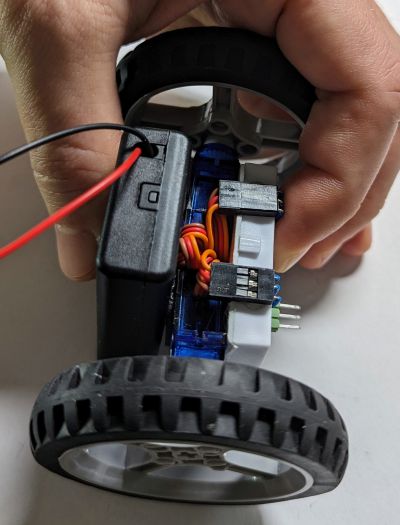
 number two: it is not a real robot, unless it has a programmable brain, like a microcontroller. But which microcontroller is the best for a beginner in year 2024? Some fifteen years ago the answer would certainly have the "Arduino" keyword in it. Nowadays, I'd say, the magic keyword is "CircuitPython". Programming just cannot get any simpler than plugging it into your computer and editing
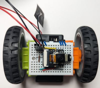
 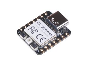 CircuitPython it is, but what specific CircuitPython-compatible microcontroller should we choose? We need something cheap and well-supported by the manufacturer and the community. The Raspberry Pi Pico would be a great match due to its popularity, price and feature set, except it is a bit too bulky (as will become clear below). Check out the Seeedstudio Xiao Series instead. The Xiao RP2040 is built upon the same chip as the Raspberry Pi Pico, is just as cheap, but has a more compact size. Interestingly, as there is a whole series of pin-compatible boards with the same shape, we can later try other models if we do not like this one. Moreover, we are not even locked into a single vendor, as the QT Py series from Adafruit is also sharing the same form factor. How cool is that? (I secretly hope this particular footprint would get more adoption by other manufacturers).
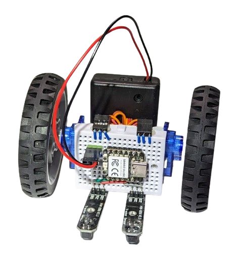
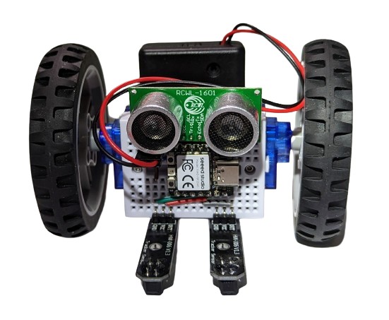
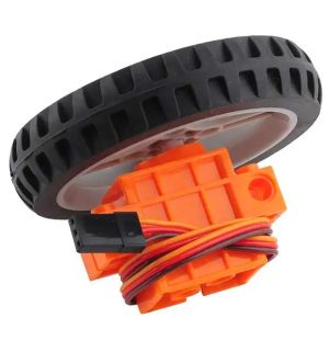
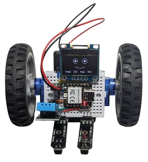 The one on the image above also had the DHT11 sensor plugged into it, so it shows humidity and temperature while it is doing its line following. Why? Because it can!
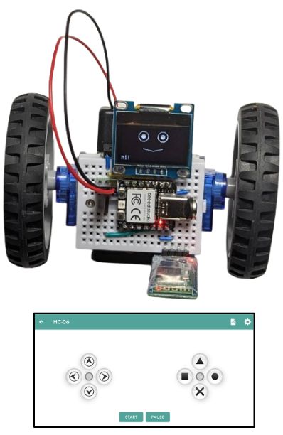
 Presenting is hard. Although I have had the opportunity to give hundreds of talks and lectures on various topics and occasions by now, preparing every new presentation still takes me a considerable amount of effort. I have had a fair share of positive feedback, though, and have developed a small set of principles which, I believe, are key to preparing (or at least learning to prepare) good presentations. Let me share them with you.
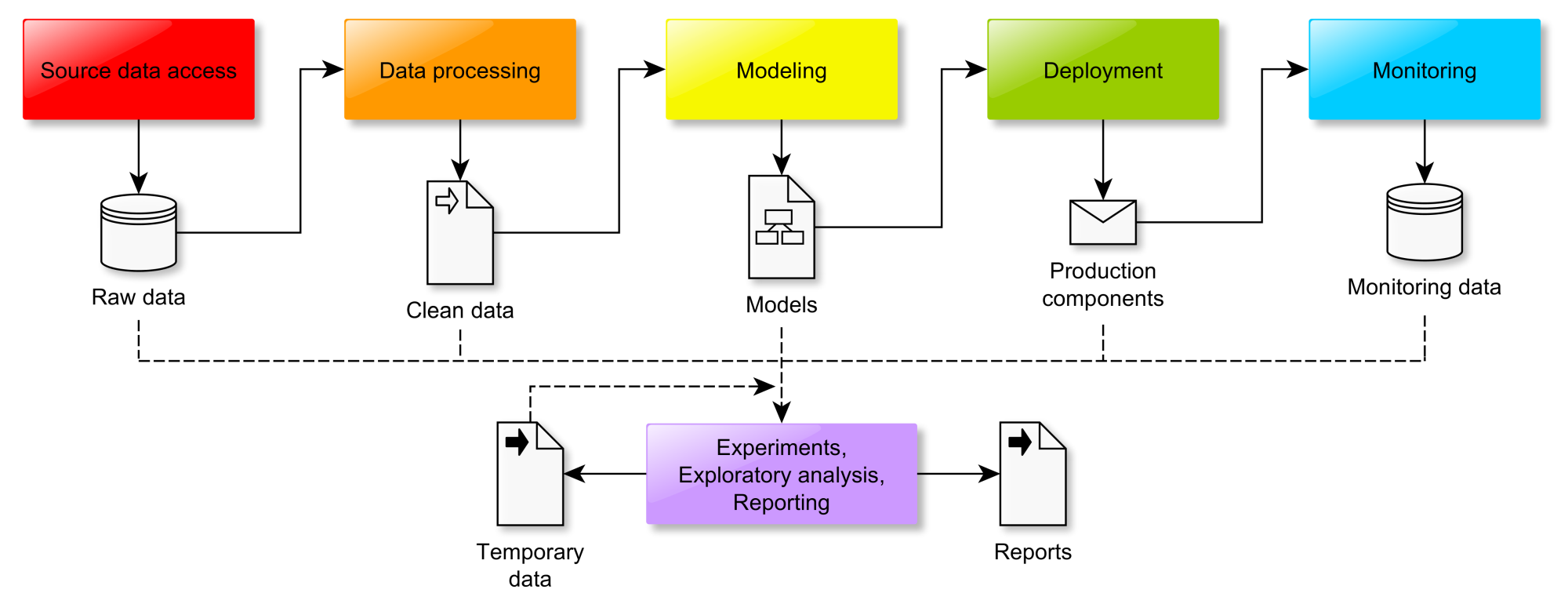


 from a normal distribution with unit covariance and we need to estimate the mean
  of this distribution.
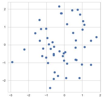
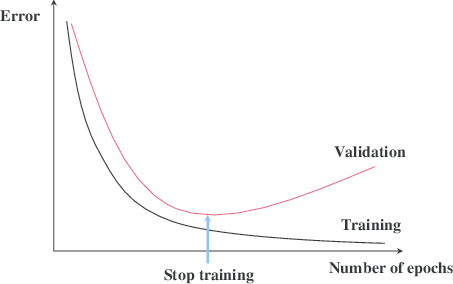
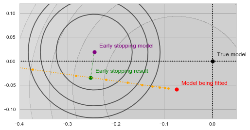
![\[f_\mathrm{train}(\mathrm{w}) := \sum_{i=1}^{50} \Vert \mathbf{x}_i - \mathbf{w}\Vert^2\]](https://fouryears.eu/wp-content/ql-cache/quicklatex.com-4a4ff04b2699f9033f5d09897e4dfc5e_l3.png "Rendered by QuickLaTeX.com")

![\[f_\mathrm{fit}(\mathrm{w}) := \sum_{i=1}^{40} \Vert \mathbf{x}_i - \mathbf{w}\Vert^2\]](https://fouryears.eu/wp-content/ql-cache/quicklatex.com-5adb94ca761b724a00c38b830a6bd831_l3.png "Rendered by QuickLaTeX.com")
![\[f_\mathrm{stop}(\mathrm{w}) := \sum_{i=41}^{50} \Vert \mathbf{x}_i - \mathbf{w}\Vert^2.\]](https://fouryears.eu/wp-content/ql-cache/quicklatex.com-8ac10bff72d2e3925e207369119b4537_l3.png "Rendered by QuickLaTeX.com")
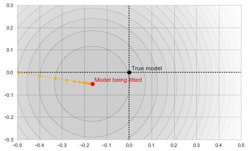
 at each step along the way:
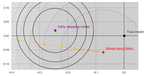
 nor of
  , and are thus inherently a worse representation of the problem altogether.
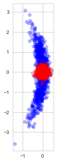
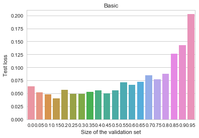
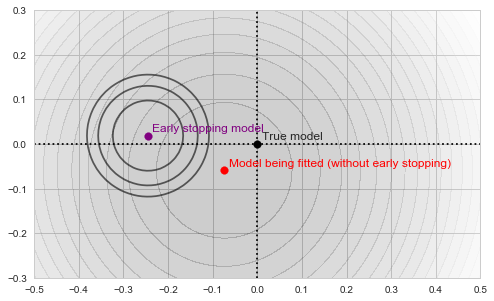
 regularization.
 -penalty added to the objective:
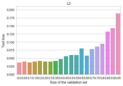
 numbers is a task that requires at least
  time in general. There are some special cases, such as sorting small integers, where you can use
  -bit number
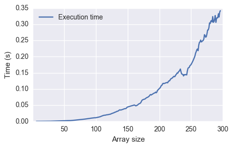
 -bit
-bit  into a
  algorithm (with
  memory consumption). This is a nice illustration of how the same algorithm can have different complexity based on the chosen execution model.
 by hashing the last block data with its own identifier. If this number is smaller than
![\[\alpha \cdot \text{(account balance)}\cdot \text{(time since last block)},\]](https://fouryears.eu/wp-content/ql-cache/quicklatex.com-1b685682ff93b14ab8bb39843ed2769f_l3.png "Rendered by QuickLaTeX.com")
 is a block-specific constant), the node gets the right to sign the next block. The higher the node's balance, the higher is the probability it will get a chance to sign. The rationale is that nodes with larger balances have more at stake, are more motivated to behave honestly, and thus need to be given more opportunities to participate in generating the blockchain.


