Four Years Remaining

This article has been cross-posted to Hackster.

What is the best way to learn (or teach) introductory robotics? What could be the "hello world" project in this field, that would be simple for a beginner to get started with, complex enough to be exciting and qualify as a "robot", and deep enough to allow further creative extensions and experiments? Let us try solving this problem logically, step by step!

First things first: what is a "robot"?

Axiom number one: for anything to feel like a robot, it must have some moving parts. Ideally, it could have the freedom move around, and probably the easiest way to achieve that would be to equip it with two wheels. Could concepts other than a two-wheeler qualify as the simplest robot? Perhaps, but let us proceed with this one as a reasonably justified assumption.

The wheels

To drive the two upcoming wheels we will need two motors along with all that driver circuitry, ugh! But wait, what about those small continuous rotation servos! They are simple, cheap, and you just need to wire them to a single microcontroller pin. Some of them are even conveniently sold along with with a LEGO-style wheel!

The microcontroller

Rule number two: it is not a real robot, unless it has a programmable brain, like a microcontroller. But which microcontroller is the best for a beginner in year 2024? Some fifteen years ago the answer would certainly have the "Arduino" keyword in it. Nowadays, I'd say, the magic keyword is "CircuitPython". Programming just cannot get any simpler than plugging it into your computer and editing code.py on the newly appeared external drive. No need for "compiling", "flashing" or any of the "install these serial port drivers to fix obscure error messages" user experiences (especially valuable if you need to give a workshop at a school computer class). Moreover, the code to control a wheel looks as straightforward as motor.throttle = 0.5.

OK, CircuitPython it is, but what specific CircuitPython-compatible microcontroller should we choose? We need something cheap and well-supported by the manufacturer and the community. The Raspberry Pi Pico would be a great match due to its popularity, price and feature set, except it is a bit too bulky (as will become clear below). Check out the Seeedstudio Xiao Series instead. The Xiao RP2040 is built upon the same chip as the Raspberry Pi Pico, is just as cheap, but has a more compact size. Interestingly, as there is a whole series of pin-compatible boards with the same shape, we can later try other models if we do not like this one. Moreover, we are not even locked into a single vendor, as the QT Py series from Adafruit is also sharing the same form factor. How cool is that? (I secretly hope this particular footprint would get more adoption by other manufacturers).

The body

OK, cool. We have our wheels and a microcontroller to steer them. We now need to build the body for our robot and wire things together somehow. What would be the simplest way to achieve that?

Let us start with the wiring, as here we know an obviously correct answer - a breadboard. No simpler manual wiring technology has been invented so far, right? Which breadboard model and shape should we pick? This will depend on how we decide to build the frame for our robot, so let us put this question aside for a moment.

How do we build the frame? The options seem infinite: we can design it in a CAD tool and laser cut it from acrylic sheets, print on a 3D printer, use some profile rails, wooden blocks, LEGO bricks,... just ask Google for some inspiration:

Ugh, this starts to feel too complicated and possibly inaccessible to a normal schoolkid.... But wait, what is it there on the back of our breadboard? Is it sticky tape? Could we just... stick... our motors to it directly and use the breadboard itself as the frame?

If we now try out a few breadboard models, we will quickly discover that the widespread, "mini-sized", 170-pin breadboard has the perfect size to host our two servos:

By an extra lucky coincindence, the breadboard even has screw holes in the right places to properly attach the motors! If we now hot glue the servo connectors to the side as shown above, we can wire them comfortably, just as any other components on the breadboard itself. Finally, there is just enough space in the back to pack all the servo wires and stick a 3xAAA battery box, which happens to be enough to power both our servos and the Xiao RP2040:

This picture shows the FS90R servos. These work just as well as the GeekServo ones shown in in the picture above.

... and thus, the BreadboardBot is born! Could a breadboard with two motors and a battery stuck to its back qualify as the simplest, lowest-tech ever robot platform? I think it could. Note that the total cost of this whole build, including the microcontroller is under $20 (under $15 if you order at the right discounts from the right places).

But what can it do?

Line following

Rule number 3: it is not a real robot if it is not able to sense the environment and react to it somehow. Hence, we need some sensors, preferably ones that would help us steer the robot (wheels are our only "actuators" so far). What are the simplest steering techniques in introductory robotics? I'd say line following and obstacle avoidance!

Let us do line following first then. Oh, but how do we attach the line tracking sensors, we should have built some complicated frame after all, right? Nope, by a yet another happy design coincidence, we can just plug them right here into our breadboard:

Thanks to the magic of CircuitPython, all it takes now to teach our robot to (even if crudely) follow a line is just three lines of code (boilerplate definitions excluded):

while True:
  servo_left.throttle = 0.1 * line_left.value
  servo_right.throttle = -0.1 * line_right.value

Obstacle avoidance

OK, a line follower implemented with a three-line algorithm is cool, can we do anything else? Sure, look how conveniently the ultrasonic distance sensor fits onto our breadboard:

Add a few more lines of uncomplicated Python code and you get a shy robot that can follow a line but will also happily go roaming around your room, steering away from any walls or obstacles:

Note how you can hear the sonar working in the video (not normally audible).

... and more

There is still enough space on the breadboard to add a button and a buzzer:

.. or splash some color with a Xiao RGB matrix:

.. or plug in an OLED screen to give your BreadboardBot a funny animated face:
The one on the image above also had the DHT11 sensor plugged into it, so it shows humidity and temperature while it is doing its line following. Why? Because it can!

Tired of programming and just want a remote-controllable toy? Sure, plug in a HC06 bluetooth serial module, program one last time, and go steer the robot yourself with a smartphone:

Other microcontroller boards, BLE, Wifi and FPV

Xiao RP2040 is great, but it has no built-in wireless connectivity! Plug in its ESP32-based cousin Xiao ESP32S3 and you can steer your robot with a Bluetooth gamepad, or via Wifi, by opening a webpage served by the robot itself!
If you have the Xiao ESP32S3 Sense (the version with a microphone and camera), that webpage can even show you the live first-person view feed of the robot's camera (conveniently positioned to look forward):

In case you were wondering, the resulting FPV bot is not a very practical solution for spying on your friends, as the microcontroller heats up a lot and consumes the battery way too fast, but it is still a fun toy and an educational project.

Finally, although the Xiao boards fit quite well with all other gadgets on the mini breadboard you are not limited by that choice either and can try plugging in any other appropriately-sized microcontroller board. Here is, for example, a BreadboardBot with an M5Stack Atom Lite running a line-follower program implemented as an ESPHome config (which you can flash over the air!).

Conclusion

The examples above are just the tip of the iceberg. Have any other sensors lying around from those "getting started with Arduino" kits that you did not find sufficiently exciting uses for so far? Maybe plugging them into the BreadboardBot is the chance to shine they were waiting for all this time! Teaching the robot to recognize familiar faces and follow them? Solving a maze? Following voice commands? Self-balancing? Programming coordinated movement of multiple robots? Interfacing the robot with your smart home or one of these fancy AI chatbots? Organizing competitions among multiple BreadboardBots? Vacuuming your desk? The sky (and your free time) is the limit here!

Consider making one and spreading the joy of breadboard robotics!

Detailed build instructions along with wiring diagrams and example code are available on the project's Github page. Contributions are warmly welcome!

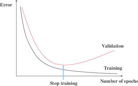
Early stopping is a technique that is very often used when training neural networks, as well as with some other iterative machine learning algorithms. The idea is quite intuitive - let us measure the performance of our model on a separate validation dataset during the training iterations. We may then observe that, despite constant score improvements on the training data, the model's performance on the validation dataset would only improve during the first stage of training, reach an optimum at some point and then turn to getting worse with further iterations.

The early stopping principle

It thus seems reasonable to stop training at the point when the minimal validation error is achieved. Training the model any further only leads to overfitting. Right? The reasoning sounds solid and, indeed, early stopping is often claimed to improve generalization in practice. Most people seem to take the benefit of the technique for granted. In this post I would like to introduce some skepticism into this view or at least illustrate that things are not necessarily as obvious as they may seem from the diagram with the two lines above.

How does Early Stopping Work?

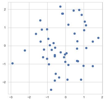
To get a better feeling of what early stopping actually does, let us examine its application to a very simple "machine learning model" - the estimation of the mean. Namely, suppose we are given a sample of 50 points from a normal distribution with unit covariance and we need to estimate the mean of this distribution.

Sample

The maximum likelihood estimate of can be found as the point which has the smallest sum of squared distances to all the points in the sample. In other words, "model fitting" boils down to finding the minimum of the following objective function:

As our estimate is based on a finite sample, it, of course, won't necessarily be exactly equal to the true mean of the distribution, which I chose in this particular example to be exactly (0,0):

Sample mean as a minimum of the objective function

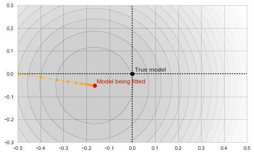
The circles in the illustration above are the contours of the objective function, which, as you might guess, is a paraboloid bowl. The red dot marks its bottom and is thus the solution to our optimization problem, i.e. the estimate of the mean we are looking for. We may find this solution in various ways. For example, a natural closed-form analytical solution is simply the mean of the training set. For our purposes, however, we will be using the gradient descent iterative optimization algorithm. It is also quite straightforward: start with any point (we'll pick (-0.5, 0) for concreteness' sake) and descend in small steps downwards until we reach the bottom of the bowl:

Gradient descent

Let us now introduce early stopping into the fitting process. We will split our 50 points randomly into two separate sets: 40 points will be used to fit the model and 10 will form the early stopping validation set. Thus, technically, we now have two different objective functions to deal with:

and

Each of those defines its own "paraboloid bowl", both slightly different from the original one (because those are different subsets of data):

Fitting and early stopping objectives

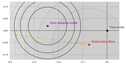
As our algorithm descends towards the red point, we will be tracking the value of at each step along the way:

Gradient descent with validation

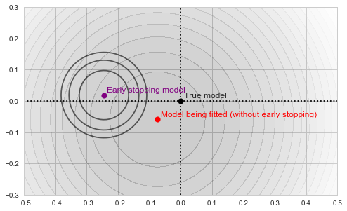
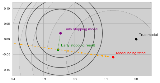
With a bit of imagination you should see on the image above, how the validation error decreases as the yellow trajectory approaches the purple dot and then starts to increase after some point midway. The spot where the validation error achieves the minimum (and thus the result of the early stopping algorithm) is shown by the green dot on the figure below:

Early stopping

In a sense, the validation function now acts as a kind of a "guardian", preventing the optimization from converging towards the bottom of our main objective. The algorithm is forced to settle on a model, which is neither an optimum of nor of . Moreover, both  and use less data than , and are thus inherently a worse representation of the problem altogether.

So, by applying early stopping we effectively reduced our training set size, used an even less reliable dataset to abort training, and settled on a solution which is not an optimum of anything at all. Sounds rather stupid, doesn't it?

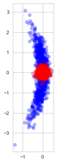
Indeed, observe the distribution of the estimates found with (blue) and without (red) early stopping in repeated experiments (each time with a new random dataset):

Solutions found with and without early stopping

As we see, early stopping greatly increases the variance of the estimate and adds a small bias towards our optimization starting point.

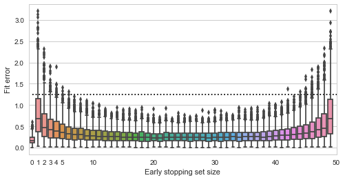
Finally, let us see how the quality of the fit depends on the size of the validation set:

Fit quality vs validation set size

Here the y axis shows the squared distance of the estimated point to the true value (0,0), smaller is better (the dashed line is the expected distance of a randomly picked point from the data).  The x axis shows all possible sizes of the validation set. We see that using no early stopping at all (x=0) results in the best expected fit. If we do decide to use early stopping, then for best results we should split the data approximately equally into training and validation sets. Interestingly, there do not seem to be much difference in whether we pick 30%, 50% or 70% of data for the validation set - the validation set seems to play just as much role in the final estimate as the training data.

Early Stopping with Non-convex Objectives

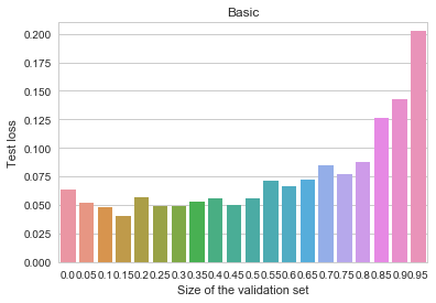
The experiment above seems to demonstrate that early stopping should be almost certainly useless (if not harmful) for fitting simple convex models. However, it is never used with such models in practice. Instead, it is most often applied to the training of multilayer neural networks. Could it be the case that the method somehow becomes useful when the objective is highly non-convex? Let us run a small experiment, measuring the benefits of early stopping for fitting a convolutional neural-network on the MNIST dataset. For simplicity, I took the standard example from the Keras codebase, and modified it slightly. Here is the result we get when training the the most basic model:

MNIST - Basic

The y axis depicts log-loss on the 10k MNIST test set, the x axis shows the proportion of the 60k MNIST training set set aside for early stopping. Ignoring small random measurement noise, we may observe that using early stopping with about 10% of the training data does seem to convey a benefit. Thus, contrary to our previous primitive example, when the objective is complex, early stopping does work as a regularization method. Why and how does it work here? Here's one intuition I find believable (there are alternative possible explanations and measurements, none of which I find too convincing or clear, though): stopping the training early prevents the algorithm from walking too far away from the initial parameter values. This limits the overall space of models and is vaguely analogous to suppressing the norm of the parameter vector. In other words, early stopping resembles an ad-hoc version of  regularization.

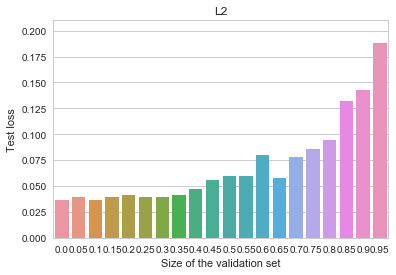
Indeed, observe how the use of early stopping affects the results of fitting the same model with a small -penalty added to the objective:

MNIST - L2

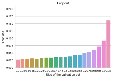
All of the benefits of early stopping are gone now, and the baseline (non-early-stopped, -regularized) model is actually better overall than it was before. Let us now try an even more heavily regularized model by adding dropout (instead of the penalty), as is customary for deep neural networks. We can observe an even cleaner result:

MNIST - Dropout

Early stopping is again not useful at all, and the overall model is better than all of our previous attempts.

Conclusion: Do We Need Early Stopping?

Given the reasoning and the anecdotal experimental evidence above, I personally tend to think that beliefs in the usefulness of early stopping (in the context of neural network training) may be well overrated. Even if it may improve generalization for some nonlinear models, you would most probably achieve the same effect more reliably using other regularization techniques, such as dropout or a simple penalty.

Note, though, that there is a difference between early stopping in the context of neural networks and, say, boosting models. In the latter case early stopping is actually more explicitly limiting the complexity of the final model and, I suspect, might have a much more meaningful effect. At least we can't directly carry over the experimental examples and results in this blog post to that case.

Also note, that no matter whether early stopping helps or harms the generalization of the trained model, it is still a useful heuristic as to when to stop a lengthy training process automatically if we simply need results that are good enough.

I happen to use the Amazon cloud machines from time to time for various personal and work-related projects. Over the years I've accumulated a terabyte or so of data files there. Those are mostly useless intermediate results or expired back-ups, which should be deleted and forgotten, but I could not gather the strength for that. "What if those datafiles happen to be of some archaelogical interest 30 years from now?", I thought. Keeping them just lying there on an Amazon machine is, however, a waste of money - it would be cheaper to download them all onto a local hard drive and tuck it somewhere into a dark dry place.

But what would be the fastest way to download a terabyte of data from the cloud? Obviously, large downstream bandwidth is important here, but so should be a smart choice of the transfer technology. To my great suprise, googling did not provide me with a simple and convincing answer. A question posted to StackOverflow did not receive any informative replies and even got downvoted for reasons beyond my understanding. It's year 2017, but downloading a file is still not an obvious matter, apparently.

Unhappy with such state of affairs I decided to compare some of the standard ways for downloading a file from a cloud machine. Although the resulting measurements are very configuration-specific, I believe the overall results might still generalize to a wider scope.

Experimental Setup

Consider the following situation:

• An m4.xlarge AWS machine (which is claimed to have "High" network bandwidth) located in the EU (Ireland) region, with an SSD storage volume (400 Provisioned IOPS) attached to it.
• A 1GB file with random data, generated on that machine using the following command:
  $ dd if=/dev/urandom of=file.dat bs=1M count=1024
• The file needs to be transferred to a university server located in Tartu (Estonia). The server has a decently high network bandwidth and uses a mirrored-striped RAID for its storage backend.

Our goal is to get the file from the AWS machine into the university server in the fastest time possible. We will now try eight different methods for that, measuring the mean transfer time over 5 attempts for each method.

File Download Methods

One can probably come up with hundreds of ways for transferring a file. The following eight are probably the most common and reasonably easy to arrange.

1. SCP (a.k.a. SFTP)

• Server setup: None (the SSH daemon is usually installed on a cloud machine anyway).
• Client setup: None (if you can access a cloud server, you have the SSH client installed already).
• Download command:
  

  scp -i ~/.ssh/id_rsa.amazon \
           ubuntu@$REMOTE_IP:/home/ubuntu/file.dat .

2. RSync over SSH

• Server setup: sudo apt install rsync (usually installed by default).
• Client setup: sudo apt install rsync (usually installed by default).
• Download command:
  

  rsync -havzP --stats \
        -e "ssh -i $HOME/.ssh/id_rsa.amazon" \
        ubuntu@$REMOTE_IP:/home/ubuntu/file.dat .

3. Pure RSync

• Server setup:
  Install RSync (usually already installed):

  sudo apt install rsync

  Create /etc/rsyncd.conf with the following contents:

  pid file = /var/run/rsyncd.pid
  lock file = /var/run/rsync.lock
  log file = /var/log/rsync.log
  
  [files]
  path = /home/ubuntu

  Run the RSync daemon:

  sudo rsync --daemon

• Client setup: sudo apt install rsync (usually installed by default).
• Download command:
  

  rsync -havzP --stats \
        rsync://$REMOTE_IP/files/file.dat .

4. FTP (VSFTPD+WGet)

• Server setup:
  Install VSFTPD:

  sudo apt install vsftpd

  Edit /etc/vsftpd.conf:

  listen=YES
  listen_ipv6=NO
  pasv_address=52.51.172.88   # The public IP of the AWS machine

  Create password for the ubuntu user:

  sudo passwd ubuntu

  Restart vsftpd:

  sudo service vsftpd restart

• Client setup: sudo apt install wget (usually installed by default).
• Download command:
  

  wget ftp://ubuntu:somePassword@$REMOTE_IP/file.dat

5. FTP (VSFTPD+Axel)

Axel is a command-line tool which can download through multiple connections thus increasing throughput.

• Server setup: See 4.
• Client setup: sudo apt install axel
• Download command:
  

  axel -a ftp://ubuntu:somePassword@$REMOTE_IP/home/ubuntu/file.dat

6. HTTP (NginX+WGet)

• Server setup:
  Install NginX:

  sudo apt install nginx

  Edit /etc/nginx/sites-enabled/default, add into the main server block:

  location /downloadme {
      alias /home/ubuntu;
      gzip on;
  }

  Restart nginx:

  sudo service nginx restart

• Client setup: sudo apt install wget (usually installed by default).
• Download command:
  

  wget http://$REMOTE_IP/downloadme/file.dat

7. HTTP (NginX+Axel)

• Server setup: See 6.
• Client setup: sudo apt install axel
• Download command:
  

  axel -a http://$REMOTE_IP/downloadme/file.dat

8. AWS S3

The last option we try is first transferring the files onto an AWS S3 bucket, and then downloading from there using S3 command-line tools.

• Server setup:
  Install and configure AWS command-line tools:

  sudo apt install awscli
  aws configure

  Create an S3 bucket:

  aws --region us-east-1 s3api create-bucket \
      --acl public-read-write --bucket test-bucket-12345 \
      --region us-east-1

  We create the bucket in the us-east-1 region because the S3 tool seems to have a bug at the moment which prevents from using it in the eu regions.

  Next, we transfer the file to the S3 bucket:

  aws --region us-east-1 s3 cp file.dat s3://test-bucket-12345

• Client setup:
  Install and configure AWS command-line tools:

  sudo apt install awscli
  aws configure

• Download command:
  

  aws --region us-east-1 s3 cp s3://test-bucket-12345/file.dat .

Results

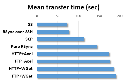
Here are the measurement results. In case of the S3 method we report the total time needed to upload from the server to S3 and download from S3 to the local machine. Note that I did not bother to fine-tune any of the settings - it may very well be possible that some of the methods can be sped up significantly by configuring the servers appropriately. Consider the results below to indicate the "out of the box" performance of the corresponding approaches.

Although S3 comes up as the fastest method (and might be even faster if it worked out of the box with the european datacenter), RSync is only marginally slower, yet it is easier to use, requires usually no additional set-up and handles incremental downloads very gracefully. I would thus summarize the results as follows:

Whenever you need to download large files from the cloud, consider RSync over SSH as the default choice.

While writing the previous post I was thinking of coming up with a small fun illustration for Aframe. I first heard about AFrame at the recent European Innovation Academy - a team-project-based entrepreneurship summer school. The team called MemVee was aiming to develop an AFrame-based site which would allow students to design and view interactive "Memory Palaces" - three-dimensional spaces with various objects related to their current study topics, organized in a way that simplifies remembering things for visual learners. Although I have never viewed a "Memory Palace" as something beyond a fantastic concept from a Sherlock Holmes TV episode, I am a visual learner myself and understand the importance of such illustrations. In fact, I try to use and preach graphical references in my teaching practice whenever I find the time and opportunity:

• In this lecture the concept of a desk is used as a visual metaphor of "structuring the information" as well as to provide an outline to the talk.
• Here and here an imaginary geographical map is used in a similar context.
• For the computer graphics course I had to develop some "slides" as small OpenGL apps for visualizing the concepts during the lecture. This has been later taken to extreme heights in the practical materials designed by Raimond-Hendrik, who went on to give this course (alongside with a seminar) in the following years. Unfortunately the materials are closed for non-participants (yet I still hope they will be opened some day, do you read this, Raimond?), but the point is that every single notion has a tiny WebGL applet made to illustrate it interactively.
• Once I tried to make a short talk about computer graphics, where the slides would be positioned on the walls of a 3D maze, so that to show them I'd have to "walk through the maze", like in a tiny first-person shooter game. Although this kind of visualization was not at all useful as a learning aid (as it did not structure anything at all), it none the less looked cool and was very well appreciated by the younger audience of the talk, to whom it was aimed at.

I have lost the sources of that last presentation to a computer error and decided to recreate a similar "maze with slides" with AFrame. The night was long and I got sucked into the process to the point of making an automated tool. You upload your slides, and it generates a random maze with your slides hanging on the walls. It is utterly useless, but the domain name "slideamaze.com" was free and I could not resist the pun. [Update from 2018 - the domain expired and the project migrated to slideamaze.ing.ee.]

Check it out. If you are into programming-related procrastination, try saving the "mazes" generated by the tool on your computer and editing the A-frame code to, say, add monsters or other fun educational tools into the maze.

Collecting large amounts of data and then using it to "teach" computers to automatically recognize patterns is pretty much standard practice nowadays. It seems that, given enough data and the right methods, computers can get quite precise at detecting or predicting nearly anything, whether it is face recognition, fraud detection or movie recommendations.

Whenever a new classification system is created, it is taken for granted that the system should be as precise as possible. Of course, classifiers that never make mistakes are rare, but if it possible, we should strive to have them make as few mistakes as possible, right? Here is a fun example, where things are not as obvious.

Consider a bank, which, as is normal for a bank, makes money by giving loans to its customers. Of course, there is always a risk that a customer will default (i.e. not repay the loan). To account for that, the bank has a risk scoring system which, for a given loan application, assesses the probability that the corresponding customer may default. This probability is later used to compute the interest rate offered for the customer. To simplify a bit, the issued interest on a loan might be computed as the sum of customer's predicted default risk probability and a fixed profit margin. For example, if a customer is expected to default with probability 10% and the bank wants 5% profit on its loans on average, the loan might be issued at slightly above 15% interest. This would cover both the expected losses due to non-repayments as well as the profit margin.

Now, suppose the bank managed to develop a perfect scoring algorithm. That is, each application gets a rating of either having 0% or 100% risk. Suppose as well that within a month the bank processes 1000 applications, half of which are predicted to be perfectly good, and half - perfectly bad. This means that 500 loans get issued with a 5% interest rate, while 500 do not get issued at all.

Think what would happen, if the system would not do such a great job and confused 50 of the bad applications with the good ones? In this case 450 applications would be classified as "100%" risk, while 550 would be assigned a risk score of "9.1%" (we still require the system to provide valid risk probability estimates). In this case the bank would issue a total of 550 loans at 15%. Of course, 50 of those would not get repaid, yet this loss would be covered from the increased interest paid by the honest lenders. The financial returns are thus exactly the same as with the perfect classifier. However, the bank now has more clients. More applications were signed, and more contract fees were received.

True, the clients might be a bit less happy for getting a higher interest rate, but assuming they were ready to pay it anyway, the bank does not care. In fact, the bank would be more than happy to segment its customers by offering higher interest rates to low-risk customers anyway. It cannot do it openly, though. The established practices usually constrain banks to make use of "reasonable" scorecards and offer better interest rates to low-risk customers.

Hence, at least in this particular example, a "worse" classifier is in fact better for business. Perfect precision is not really the ultimately desired feature. Instead, the system is much more useful when it provides a relevant and "smooth" distribution of predicted risk scores, making sure the scores themselves are decently precise estimates for the probability of a default.

The developments of proper GPU-based implementations of neural network training methods in the recent years have lead to a steady growth of exciting practical examples of their potential. Among others, the topic of face recognition (not to be confused with face detection) is on the steady rise. Some 5 years ago or so, decent face recognition tools were limited to Google Picasa and Facebook, some research labs and a few commercial products, often branded with the word "Biometrics" (that somehow seems to grow out of fashion nowadays).

Today things are different. Given a decently large labeled dataset, some knowledge of machine learning, familiarity with the GPU-based "deep learning" tools, and sufficient perseverence, one can design a reasonably impressive face recognizer system in a matter of several weeks or months at most. Consequently, now is the time when we can see recognition-based startups receive millions in funding. Just some months ago Microsoft came out with their own public face detection and recognition API (which got its fair share of publicity in the form of a funny age-guessing tool).

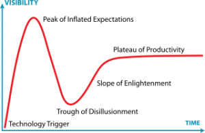
The Hype Cycle

Hence, the growth in popularity and use of face recognition is apparent. Given that the initially overinflated hype around the whole deep learning buzzword seems to have more-or-less settled down to reality, this time the growth is realistic. We are probably on the "enlightenment" segment of the hype cycle here, very close to reaching actual productivity (which is not without issues, though).

Tambet and Ardi of our institute's neuroscience research group seemed to have caught the noospheric trend and are working on a neural-network based face recognizer with the initial aim of using it to sort and organize historical photos from the Estonian National Archives.

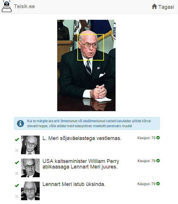
During a Skype University Hackathon, which happened in April I had the chance to join forces with them to present their efforts in the form of a fun public web app. The idea was to let people search for similar faces in the Estonian archive photos. The resulting site was called "teisik.ee" ("doppelganger" in Estonian). Although it does not seem to exactly fulfil the "doppelganger finding" purpose, it does manage to identify persons known to the system from the database surprisingly well.

Output from teisik.ee

Having observed that finding matches to celebrities, even if they are not perfect matches, is entertaining in its own way, we also managed to put up a second version of the service (all within that same weekend!), codenamed celebritymatch.me. This app lets you search the dataset of celebrity faces for those which are apparently similar (according to the opinion of our neural network, at least). Try it, it is not perfect, but rather fun.

The implementation of the recognition system is rather straightforward for anyone who knows what a convolutional network is and otherwise pretty impossible to grasp in full, hence I won't go into much technical detail. It is implemented using Caffe and consists of three consequtive convolutional layers (with ReLU and max-pooling), followed by a fully-connected hidden layer, which is then fully-connected to a softmax classification output layer. The outputs of the penultimate layer (of size 64) are used as the feature representation of the face. Those feature representations are then used to find Euclidean-distance-wise nearest neighbors in the database of faces. The future plans are to later apply the probably smarter FaceNet approach to network training for the same use case. The webapp is done using Flask.

Right after the hackathon Tambet was invited to give an interview about the project on Estonian television. If you understand Estonian, check it out, it is very good.

"Hello world" in Flask

Over the recent years I happen to have made several small personal projects using Python's Flask web framework. The framework is designed to provide a very minimalistic "bottom-up" approach. It feels slightly less cluttered and imposing than some of the popular alternatives, thus fitting nicely for the projects a single person might typically want to hack up in a spare weekend. Minimalism of Flask does not mean it is somehow limited or unsuitable for larger projects - perhaps on the contrary, small size of the framework means there are fewer restrictions on what and how you can do with it.

What a small framework needs to be applied comfortably beyond its 6-line "Hello-World" use case, however, is a decent starter project template that would include some of the most common bells and whistles. And indeed, there happen to be several such templates available. I used parts of them over time in my own projects, however I always ended redoing/rewriting/renaming bits and pieces to fit my personal aesthetic needs. Eventually I got tired of renaming and packaged a Flask application template in the way I consistently prefer to use it. I am not sure whether it is objectively better or worse than the alternatives. None the less, if at some point you decide to give Flask a try, let me suggest you try this template of mine as your point of origin.

When it comes to data analysis, there are hundreds of exciting approaches: simple summary statistics and hypothesis tests, various clustering methods, linear and nonlinear regression or classification techniques, neural networks of various types and depths, decision rules and frequent itemsets, feature extractors and dimension reductors, ensemble methods, bayesian approaches and graphical models, logic-based approaches and fuzzy stuff, ant colonies, genetic algorithms and other optimization methods, monte-carlo algorithms, sampling and density estimation, logic-based and graph methods. Don't even get me started on the numerous visualization techniques.

This sheer number of options is, however, both a blessing and a curse at the same time. In many practical situations just having those methods at your disposal may pose more problems than solutions. First you need to pick one of the approaches that might possibly fit your purpose. Then you will try to adapt it appropriately, spend several iterations torturing the data only to obtain very dubious first results, come to the conclusion that most probably you are doing something wrong, reconvince yourself that you need to try harder in that direction, spend some more iterations testing various parameter settings. Nothing works as you want it to, so you start everything from scratch with another method to find yourself obtaining new, even more dubious results, torturing the data even further, getting tired of that and finally settling on something "intermediately decent", which "probably makes sense", although you are not so sure any more and feel frustrated.

I guess life of a statistician was probably way simpler back in the days when you could run a couple of t-tests, or an F-test from a linear regression and call it a day. In fact, it seems that many experimental (e.g. wetlab) scientists still live in that kind of world, when it comes to analyzing their experimental results. The world of T-tests is cozy and safe. They don't get you frustrated. Unfortunately, t-tests can feel ad-hockish, because they force you to believe that something "is normally distributed". Also, in practice, they are mainly used to confirm the obvious rather than discover something new from the data. A simple scatterplot will most often be better than a t-test as an analysis method. Hence, I am not a big fan of T-tests. However, I do have my own favourite statistical method, which always feels cozy and safe, and never gets me frustrated. I tend to apply it whenever I see a chance. It is the Fisher exact test in the particular context of feature selection.

My appreciation of it stems from my background in bioinformatics and some experience with motif detection in particular. Suppose you have measured the DNA sequences for a bunch of genes. What can you do to learn something new about the sequence structure from that data? One of your best bets is to first group your sequences according to some known criteria. Suppose you know from previous experiments that some of the genes are cancer-related whereas others are not. As soon as you have specified those groups, you can start making observations like the following: "It seems that 10 out of my 20 cancer-related genes have the subsequence GATGAG in their DNA code. The same sequence is present in only 5 out of 100 non-cancer-related ones. How probable would it be to obtain similar counts of GATGAG, if the two groups were picked randomly?" If the probability to get those counts at random is very low, then obviously there is something fishy about GATGAG and cancer - perhaps they are related. To compute this probability you will need to use the hypergeometric distribution, and the resulting test (i.e. the question "how probable is this situation in a random split?") is known as the Fishers' exact test.

This simple logic (with a small addition of a multiple testing correction on top) has worked wonders for finding actually important short sequences on the DNA. Of course it is not limited to sequence search. One of our research group's most popular web tools uses the same approach to discover functional annotations, that are "significantly overrepresented" in a given group of genes. The same approach can be used to construct decision trees, and in pretty much any other "supervised learning" situation, where you have groups of objects and want to find binary features of those objects, associated with the groups.

Although in general the Fisher test is just one particular measure of association, it is, as I noted above, rather "cozy and comfortable". It does not force me to make any weird assumptions, there is no "ad-hoc" aspect to it, it is simple to compute and, most importantly, in my experience it nearly always produces "relevant" results.

Words overrepresented in the speeches of Greece MPs

A week ago me, Ilya and Alex happened to take part in a small data analysis hackathon, dedicated to the analysis of speech transcripts from the European Parliament. Somewhat analogously to DNA sequences, speeches can be grouped in various ways: you can group them by the speaker who gave them, by country, gender or political party of that speaker, by the month or year when the speech was given or by any combination of such groupings. The obvious "features" of a speech are words, which can be either present or not present in it. Once you view the problem this way the task of finding group-specific words becomes self-evident and the Fisher test is the natural solution to it. We implemented this idea and extracted "country-specific" and "time-specific" words from the speeches (other options were left out due to time constraints). As is usual the case with my favourite method, the obtained results look relevant, informative and, when shown in the form of a word cloud, fun. Check them out.

The complete source code of the analysis scripts and the visualization application is available on Github.

Update from year 2017: The tool described in this post DOES NOT WORK with recent versions of Skype. Either these versions stopped saving removed messages altogether, or they are doing it in a novel manner not recognized by the tool.

In other words - you would only recover "removed" messages if you are running older version of Skype (or these messages were sent at the time you were using that older version).

Yesterday I happened to attend a discussion about the security and privacy of information stored locally in Skype and Thunderbird profiles. It turns out, if you obtain a person's Skype profile directory, you will be able to log in as him without the need to know the password. In addition, Dominique made a remark that Skype does not really delete the messages that are marked as "removed" in the chat window. I found that curious and decided to take a closer look.

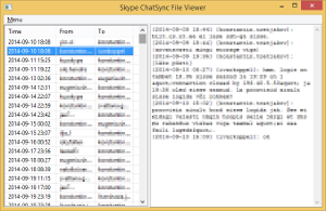
Indeed, there is a bunch of *.dat files in the chatsync subdirectory of the Skype's profile, which preserve all messages along with all their edits or deletions. Unfortunately, the *.dat files are in some undocumented binary format, and the only tool I found for reading those lacks in features. However, hacking up a small Python parser according to what is known about the format, along with a minimalistic GUI is a single evening's exercise, and I happened to be in the mood for some random coding.

Skype Chatsync Viewer

Now, if you want to check out what was that message you or your conversation partner wrote before it was edited or deleted, this package will help. If you are not keen on installing Python packages, here is a standalone Windows executable.

Despite the popularity of Python, I find that many of its best practices are not extremely well-documented. In particular, whenever it comes to starting a new Python project, quite a lot of people would follow whatever the very first Python tutorial taught them (or whatever their IDE creates), and start churning out .py files, perhaps organizing them into subdirectories along the way. This is not a good idea. Eventually they would stumble upon problems like "how do I distribute my code", "how do I manage dependencies", "where do I put documentation", "how (and when) should I start writing tests for my code", etc. Dealing with those issues "later" is always much more annoying than starting with a proper project layout in the first place.

Although there is no unique standard for a project layout, there are some established best practices. In particular (and this seems to be not very widely known), one of the easiest ways to create a new Python package (i.e., develop anything in Python that will have to be distributed later), is to make use of the paster or cookiecutter tools. Simply running

$ paster create <package_name>

or

$ cookiecutter https://github.com/audreyr/cookiecutter-pypackage.git

will ask you some questions and initialize a well-formed setuptools-based package layout for you. A slightly more involved yet still minimalistic starter code is provided by additional paster/cookiecutter templates, such as modern-package-template:

$ pip install modern-package-template
$ paster create -t modern_package <package_name>

Naturally, every developer will tend to customize the setup, by adding the necessary tools. Moreover, the preferred setup evolves with time, as various tools and services come in and out of existence. Ten years ago, buildout or git were not yet around. Five years ago, there was no tox and nose was better than py.test. Services like Travis-CI and Github are even younger yet.

Although I tend to experiment a lot with my setup, over the recent couple of years I seem to have converged to a fairly stable Python environment, which I decided to share as a reusable template and recommend anyone to make use of it.

Thus, next time you plan to start a new Python project, try beginning with:

$ pip install python_boilerplate_template
$ paster create -t python_boilerplate <project_name>

or, alternatively,

$ pip install cookiecutter
$ cookiecutter https://github.com/konstantint/cookiecutter-python-boilerplate

More information here (for paster) or here (for cookiecutter). Contributions and constructive criticism welcome via Github.