Four Years Remaining

Ever since Erwin Schrödinger described a thought experiment, in which a cat in a sealed box happened to be "both dead and alive at the same time", popular science writers have been relying on it heavily to convey the mysteries of quantum physics to the layman. Unfortunately, instead of providing any useful intuition, this example has instead laid solid base to a whole bunch of misconceptions. Having read or heard something about the strange cat, people would tend to jump to profound conclusions, such as "according to quantum physics, cats can be both dead and alive at the same time" or "the notion of a conscious observer is important in quantum physics". All of these are wrong, as is the image of a cat, who is "both dead and alive at the same time". The corresponding Wikipedia page does not stress this fact well enough, hence I thought the Internet might benefit from a yet another explanatory post.

The Story of the Cat

The basic notion in quantum mechanics is a quantum system. Pretty much anything could be modeled as a quantum system, but the most common examples are elementary particles, such as electrons or photons. A quantum system is described by its state. For example, a photon has polarization, which could be vertical or horizontal. Another prominent example of a particle's state is its wave function, which represents its position in space.

There is nothing special about saying that things have state. For example, we may say that any cat has a "liveness state", because it can be either "dead" or "alive". In quantum mechanics we would denote these basic states using the bra-ket notation as and . The strange thing about quantum mechanical systems, though, is the fact that quantum states can be combined together to form superpositions. Not only could a photon have a purely vertical polarization  or a purely horizontal polarization , but it could also be in a superposition of both vertical and horizontal states:

This means that if you asked the question "is this photon polarized vertically?", you would get a positive answer with 50% probability - in another 50% of cases the measurement would report the photon as horizontally-polarized. This is not, however, the same kind of uncertainty that you get from flipping a coin. The photon is not either horizontally or vertically polarized. It is both at the same time.

Amazed by this property of quantum systems, Schrödinger attempted to construct an example, where a domestic cat could be considered to be in the state

which means being both dead and alive at the same time. The example he came up with, in his own words (citing from Wikipedia), is the following:

A cat is penned up in a steel chamber, along with the following device (which must be secured against direct interference by the cat): in a Geiger counter, there is a tiny bit of radioactive substance, so small, that perhaps in the course of the hour one of the atoms decays, but also, with equal probability, perhaps none; if it happens, the counter tube discharges and through a relay releases a hammer that shatters a small flask of hydrocyanic acid. If one has left this entire system to itself for an hour, one would say that the cat still lives if meanwhile no atom has decayed. The first atomic decay would have poisoned it.

The idea is that after an hour of waiting, the radiactive substance must be in the state

the poison flask should thus be in the state

and the cat, consequently, should be

Correct, right? No.

The Cat Ensemble

Superposition, which is being "in both states at once" is not the only type of uncertainty possible in quantum mechanics. There is also the "usual" kind of uncertainty, where a particle is in either of two states, we just do not exactly know which one. For example, if we measure the polarization of a photon, which was originally in the superposition , there is a 50% chance the photon will end up in the state  after the measurement, and a 50% chance the resulting state will be . If we do the measurement, but do not look at the outcome, we know that the resulting state of the photon must be either of the two options. It is not a superposition anymore. Instead, the corresponding situation is described by a statistical ensemble:

Although it may seem that the difference between a superposition and a statistical ensemble is a matter of terminology, it is not. The two situations are truly different and can be distinguished experimentally. Essentially, every time a quantum system is measured (which happens, among other things, every time it interacts with a non-quantum system) all the quantum superpositions are "converted" to ensembles - concepts native to the non-quantum world. This process is sometimes referred to as decoherence.

Now recall the Schrödinger's cat. For the cat to die, a Geiger counter must register a decay event, triggering a killing procedure. The registration within the Geiger counter is effectively an act of measurement, which will, of course, "convert" the superposition state into a statistical ensemble, just like in the case of a photon which we just measured without looking at the outcome. Consequently, the poison flask will never be in a superposition of being "both broken and not". It will be either, just like any non-quantum object should. Similarly, the cat will also end up being either dead or alive - you just cannot know exactly which option it is before you peek into the box. Nothing special or quantum'y about this.

The Quantum Cat

"But what gives us the right to claim that the Geiger counter, the flask and the cat in the box are "non-quantum" objects?", an attentive reader might ask here. Could we imagine that everything, including the cat, is a quantum system, so that no actual measurement or decoherence would happen inside the box? Could the cat be "both dead and alive" then?

Indeed, we could try to model the cat as a quantum system with and being its basis states. In this case the cat indeed could end up in the state of being both dead and alive. However, this would not be its most exciting capability. Way more suprisingly, we could then kill and revive our cat at will, back and forth, by simply measuring its liveness state appropriately. It is easy to see how this model is unrepresentative of real cats in general, and the worry about them being able to be in superposition is just one of the many inconsistencies. The same goes for the flask and the Geiger counter, which, if considered to be quantum systems, get the magical abilities to "break" and "un-break", "measure" and "un-measure" particles at will. Those would certainly not be a real world flask nor a counter anymore.

The Cat Multiverse

There is one way to bring quantum superposition back into the picture, although it requires some rather abstract thinking. There is a theorem in quantum mechanics, which states that any statistical ensemble can be regarded as a partial view of a higher-dimensional superposition. Let us see what this means. Consider a (non-quantum) Schrödinger's cat. As it might be hopefully clear from the explanations above, the cat must be either dead or alive (not both), and we may formally represent this as a statistical ensemble:

It turns out that this ensemble is mathematically equivalent in all respects to a superposition state of a higher order:

where "Universe A" and "Universe B" are some abstract, unobservable "states of the world". The situation can be interpreted by imagining two parallel universes: one where the cat is dead and one where it is alive. These universes exist simultaneously in a superposition, and we are present in both of them at the same time, until we open the box. When we do, the universe superposition collapses to a single choice of the two options and we are presented with either a dead, or a live cat.

Yet, although the universes happen to be in a superposition here, existing both at the same time, the cat itself remains completely ordinary, being either totally dead or fully alive, depending on the chosen universe. The Schrödinger's cat is just a cat, after all.

Imagine a weight hanging on a spring. Let us pull the weight a bit and release it into motion. What will its motion look like? If you remember some of your high-school physics, you should probably answer that the resulting motion is a simple harmonic oscillation, best described by a sinewave. Although this is a fair answer, it actually misses an interesting property of real-life springs. A property most people don't think much about, because it goes a bit beyond the high school curriculum. This property is best illustrated by

The Slinky Drop

The "slinky drop" is a fun little experiment which has got its share of internet fame.

The Slinky Drop

When the top end of a suspended slinky is released, the bottom seems to patiently wait for the top to arrive before starting to fall as well. This looks rather unexpected. After all, we know that things fall down according to a parabola, and we know that springs collapse according to a sinewave, however neither of the two rules seem to apply here. If you browse around, you will see lots of awesome videos demonstrating or explaining this effect. There are news articles, forum discussions, blog posts and even research papers dedicated to the magical slinky. However, most of them are either too sketchy or too complex, and none seem to mention the important general implications, so let me give a shot at another explanation here.

The Slinky Drop Explained Once More

Let us start with the classical, "high school" model of a spring. The spring has some length in the relaxed state, and if we stretch it, making it longer by , the two ends of the spring exert a contracting force of . Assume we hold the top of the spring at the vertical coordinate and have it balance out. The lower end will then position at the coordinate , where the gravity force is balanced out exactly by the spring force.

How would the two ends of the spring behave if we let go off the top now? Here's how:

The horozontal axis here denotes the time, the vertical axis - is the vertical position. The blue curve is the trajectory of the top end of the spring, the green curve - trajectory of the bottom end. The dotted blue line is offset from the blue line by exactly - the length of the spring in relaxed state.

Observe that the lower end (the green curve), similarly to the slinky, "waits" for quite a long time for the top to approach before starting to move with discernible velocity. Why is it the case? The trajectory of the lower point can be decomposed in two separate movements. Firstly, the point is trying to fall down due to gravity, following a parabola. Secondly, the point is being affected by string tension and thus follows a cosine trajectory. Here's how the two trajectories look like separately:

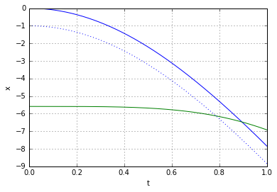
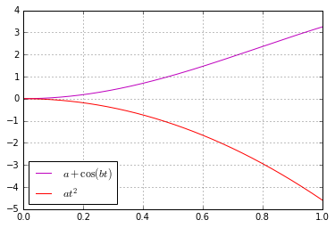
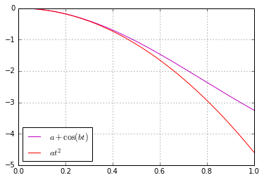
They are surprisingly similar at the start, aren't they? And indeed, the cosine function does resemble a parabola up to . Recall the corresponding Taylor expansion:

If we align the two curves above, we can see how well they match up at the beginning:

Consequently, the two forces happen to "cancel" each other long enough to leave an impression that the lower end "waits" for the upper for some time. This effect is, however, much more pronounced in the slinky. Why so?

Because, of course, a single spring is not a good model for the slinky. It is more correct to regard a slinky as a chain of strings. Observe what happens if we model the slinky as a chain of just three simple springs:

Each curve here is the trajectory of one of the nodes inbetween the three individual springs. We can see that the top two curves behave just like a single spring did - the green node waits a bit for the blue and then starts moving. The red one, however, has to wait longer, until the green node moves sufficiently far away. The bottom, in turn, will only start moving observably when the red node approaches it close enough, which means it has to wait even longer yet - by that time the top has already arrived. If we consider a more detailed model, the movement  of a slinky composed of, say, 9 basic springs, the effect of intermediate nodes "waiting" becomes even more pronounced:

To make a "mathematically perfect" model of a slinky we have to go to the limit of having infinitely many infinitely small springs. Let's briefly take a look at how that solution looks like.

The Continuous Slinky

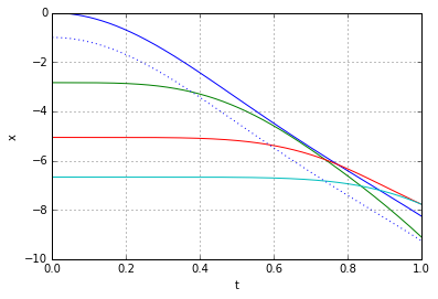
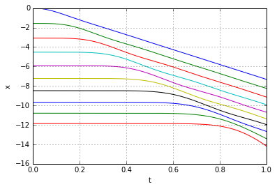
Let denote the coordinate of a point on a "relaxed" slinky. For example, in the two discrete models above the slinky had 4 and 10 points, numbered and respectively. The continuous slinky will have infinitely many points numbered .

Let denote the vertical coordinate of a point at time . The acceleration of point at time is then, by definition , and there are two components affecting it: the gravitational pull and the force of the spring.

The spring force acting on a point is proportional to the stretch of the spring at that point . As each point is affected by the stretch from above and below, we have to consider a difference of the "top" and "bottom" stretches, which is thus the derivative of the stretch, i.e. . Consequently, the dynamics of the slinky can be described by the equation:

where is some positive constant. Let us denote the second derivatives by and , replace with and rearrange to get:

(1)  

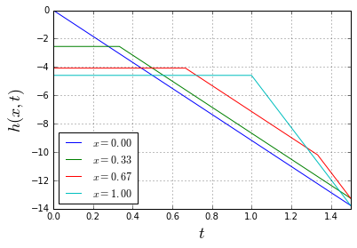
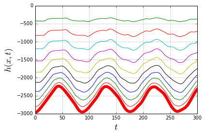
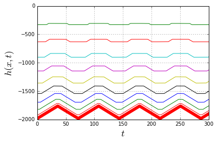
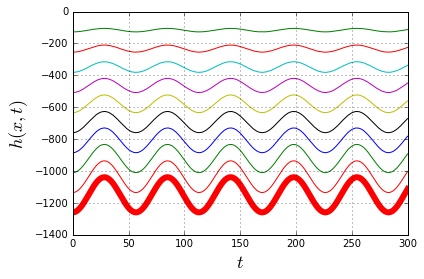
which is known as the wave equation. The name stems from the fact that solutions to this equation always resemble "waves" propagating at a constant speed through some medium. In our case the medium will be the slinky itself. Now it becomes apparent that, indeed, the lower end of the slinky should not move before the wave of disturbance, unleashed by releasing the top end, reaches it. Most of the explanations of the slinky drop seem to refer to that fact. However when it is stated alone, without the wave-equation-model context, it is at best a rather incomplete explanation.

Given how famous the equation is, it is not too hard to solve it. We'll need to do it twice - first to find the initial configuration of a suspended slinky, then to compute its dynamics when the top is released.

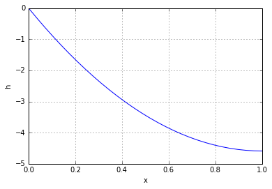
In the beginning the slinky must satisfy (because it is not moving at all), (because the top end is located at coordinate 0), and (because there is no stretch at the bottom). Combining this with (1) and searching for a polynomial solution, we get:

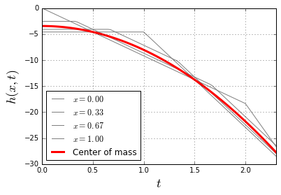
Next, we release the slinky, hence the conditions and disappear and we may use the d'Alembert's formula with reflected boundaries to get the solution:

Here's how the solution looks like visually:

Notice how the part of the slinky to which the wave has not arrived yet, stays completely fixed in place. Here are the trajectories of 4 equally-spaced points on the slinky:

Note how, quite surprisingly, all points of the slinky are actually moving with a constant speed, changing it abruptly at certain moments. Somewhat magically, the mean of all these piecewise-linear trajectories (i.e. the trajectory of the center of mass of the slinky) is still a smooth parabola, just as it should be:

The Secret of Spring Motion

Now let us come back to where we started. Imagine a weight on a spring. What will its motion be like? Obviously, any real-life spring is, just like the slinky, best modeled not as a Hooke's simple spring, but rather via the wave equation. Which means that when you let go off the weight, the weight will send a deformation wave, which will move along the spring back and forth, affecting the pure sinewave movement you might be expecting from the simple Hooke's law. Watch closely:

Here is how the movement of the individual nodes looks like:

The fat red line is the trajectory of the weight, and it is certainly not a sinewave. It is a curve inbetween the piecewise-linear "sawtooth" (which is the limit case when the weight is zero) and the true sinusoid (which is the limit case when the mass of the spring is zero). Here's how the zero-weight case looks like:

And this is the other extreme - the massless spring:

These observations can be summarized into the following obviously-sounding conclusion: the basic Hooke's law applies exactly only to the the massless spring. Any real spring has a mass and thus forms an oscillation wave traveling back and forth along its length, which will interfere with the weight's simple harmonic oscillation, making it "less simple and harmonic". Luckily, if the mass of the weight is large enough, this interference is negligible.

And that is, in my opinion, one of the interesting, yet often overlooked aspects of spring motion.

Collecting large amounts of data and then using it to "teach" computers to automatically recognize patterns is pretty much standard practice nowadays. It seems that, given enough data and the right methods, computers can get quite precise at detecting or predicting nearly anything, whether it is face recognition, fraud detection or movie recommendations.

Whenever a new classification system is created, it is taken for granted that the system should be as precise as possible. Of course, classifiers that never make mistakes are rare, but if it possible, we should strive to have them make as few mistakes as possible, right? Here is a fun example, where things are not as obvious.

Consider a bank, which, as is normal for a bank, makes money by giving loans to its customers. Of course, there is always a risk that a customer will default (i.e. not repay the loan). To account for that, the bank has a risk scoring system which, for a given loan application, assesses the probability that the corresponding customer may default. This probability is later used to compute the interest rate offered for the customer. To simplify a bit, the issued interest on a loan might be computed as the sum of customer's predicted default risk probability and a fixed profit margin. For example, if a customer is expected to default with probability 10% and the bank wants 5% profit on its loans on average, the loan might be issued at slightly above 15% interest. This would cover both the expected losses due to non-repayments as well as the profit margin.

Now, suppose the bank managed to develop a perfect scoring algorithm. That is, each application gets a rating of either having 0% or 100% risk. Suppose as well that within a month the bank processes 1000 applications, half of which are predicted to be perfectly good, and half - perfectly bad. This means that 500 loans get issued with a 5% interest rate, while 500 do not get issued at all.

Think what would happen, if the system would not do such a great job and confused 50 of the bad applications with the good ones? In this case 450 applications would be classified as "100%" risk, while 550 would be assigned a risk score of "9.1%" (we still require the system to provide valid risk probability estimates). In this case the bank would issue a total of 550 loans at 15%. Of course, 50 of those would not get repaid, yet this loss would be covered from the increased interest paid by the honest lenders. The financial returns are thus exactly the same as with the perfect classifier. However, the bank now has more clients. More applications were signed, and more contract fees were received.

True, the clients might be a bit less happy for getting a higher interest rate, but assuming they were ready to pay it anyway, the bank does not care. In fact, the bank would be more than happy to segment its customers by offering higher interest rates to low-risk customers anyway. It cannot do it openly, though. The established practices usually constrain banks to make use of "reasonable" scorecards and offer better interest rates to low-risk customers.

Hence, at least in this particular example, a "worse" classifier is in fact better for business. Perfect precision is not really the ultimately desired feature. Instead, the system is much more useful when it provides a relevant and "smooth" distribution of predicted risk scores, making sure the scores themselves are decently precise estimates for the probability of a default.

If anyone tells you he or she understands probability theory, do not believe them. That person simply does not know enough of it to admit, that probability theory is riddled with paradoxes, where common sense must step aside and wait in silence, or your brain will hurt. Substring statistics is probably among the lesser-known, yet magically unintuitive examples.

Consider a sequence of random coin flips. Each coin flip is either a "heads" or a "tails", hence the sequence might written down as a sequence of H and T-s: HTHTHHTT...

It is easy to show that the probability of the sequence to begin with, say, HHH is equal to P(HHH) = 1/8th, as is the case with any other three-letter combination: P(HHT) = P(THH) = P(THT) = 1/8, etc. Moreover, by symmetry, the probability of seeing a particular three-letter combination at any fixed position in the sequence is still always 1/8-th. All three-letter substrings seem to be equivalent here.

But let us now play a game, where we throw a coin until we see a particular three-letter combination. To be more specific, let us wait until either HHT or HHH comes up. Suppose I win in the first case and you win in the second one. Obviously, the game first proceeds until two heads are flipped. Then, whichever coin flip comes up next determines the winner. Sounds pretty fair, doesn't it? Well, it turns out that, surprisingly, if you count carefully the expected number of coin flips to obtain HHT, it happens to be 8, whereas for HHH it is 14! Ha! Does it mean I have an advantage? Suprisingly again, no. The probability of HHT occuring before HHH in any given sequence is still precisely 0.5 and, as we reasoned initially, the game is still fair.

We can, however, construct even more curious situations with four-letter combinations. Suppose I bet on HTHT and you bet on THTT.  The expected number of coin flips to obtain my combination can be computed to be 20. The expected number of flips to get your combination is smaller: 18 flips. However, it is still more probable (64%) that my combination will happen before yours!

If this is not amusing enough, suppose that four of us are playing such a game. Player A bets on the string THH, Player B bets on HHT, player C on HTT and player D on TTH. It turns out that A's combination will occur earlier than B's with probability 75%. B's combination, however, wins over C's with probability 66.7%. C's combination, though, wins over D's with probability 75%. And, to close the loop, D wins over A with probability 66.7%! This is just like the nontransitive dice.

Hopefully, you are amazed enough at this point to require an explanation for how this all might happen. Let me leave it to you as a small puzzle:

• Explain in simple terms, how can it happen so that the expected time to first occurrence of otherwise equiprobable substrings may be different?
• Explain in simple terms, how can it be so that one substring has higher than 50% chance of occuring earlier than some other substring.
• Finally, explain why the two effects above are not strictly related to each other.

PS: The theory used to compute actual probabilities and expected times to occurrence of a substring is elegant yet somewhat involved. For the practically-minded, here is the code to check the calculations.

Sportloto lottery ticket

Consider the following hypothetical lottery scheme. A player pays a dollar for a lottery ticket. On the ticket he has to mark a number between 1 and 100. When sufficient number of tickets was sold, the single "lucky number" is drawn randomly using a lotto machine, and half of the proceeds from ticket sales are shared equally among all tickets that bet on that number. The other half goes to charity.

Now, given the whole "charity" deal, the amount of money going into the lottery is greater than the amount of money paid back, hence the game is obviously disadvantageous for the players. The expected returns of an average ticket are just $0.5, hence "the house always wins", and "lottery is a tax on people who do not understand probability theory", as they say. Right? It turns out things are not that simple.

Suppose there are 100 000 people in the country who play this lottery, each one buying a single ticket. Let us imagine that, for some reason, everyone who plays the lottery is extremely superstitious and will never bet on the number 13 because it is universally despised as unlucky. Knowing that, let us now go and buy a single ticket, betting on 13. Behold: we have just paid one dollar for a 1% chance to win 50 000 dollars! Indeed, there is a 1% chance the lottery machine will draw 13 as the winning number and if this happens we will be the only candidate for receiving the whole winning fund - $50 000 in our case. Consequently, the expected returns for our ticket are $50 000 x 0.01 = $500, and the bet is well worth its price.

In general, it is easy to show that betting on any number which is sufficiently unpopular, namely any number which less than 500 of the 100 000 participants will decide to bet on, results in positive expected returns (note that on average we expect about 1000 people to bet on a "random" number).

To highlight the concept a bit more, let us consider an even better hypothetical possibility. Let us say that all of the 100 000 lottery players decide to bet on their birth dates. This means that their bets would cover only the numbers between 1 and 31. The smart idea then would be to buy 69 tickets, betting on each of the remaining numbers (32..100). Such a bet costs $69 and wins the sum of $50 034 with probability 69%. The expected returns per each dollar invested are still around $500, but in addition you win with astonishing certainty.

Does this have anything to do with reality? It turns out it does. This article from 1980 (in Russian) studies the popular Soviet lottery "Sportloto", in which the players had to select 5 or 6 numbers from a grid of 36 or 45 numbers respectively (see illustration above). The drawing was performed, and the players who managed to guess enough numbers would share a portion of the lottery fund. Note that this is just a more elaborate variation of the "pick one out of 100" lottery above. And of course, psychological aspects play a large role in biasing players' number selections. People tend to prefer numbers towards the bottom of the grid to those on the first lines. People prefer smaller numbers to larger ones. And, most importantly, people tend to avoid picking regular patterns (e.g. all numbers in a sequence, or those forming a nice rectangle), as such combinations intuitively seem to be "too improbable to happen".

This results in a situation where betting on a "psychologically improbable" pattern of numbers may turn out to be profitable in terms of expected returns. The authors of the mentioned article actually used historical lottery drawing data to estimate the returns they would have if they would constantly participate in Sportloto using such patterns, and reported the ratio of winnings to spending of around 1.15 to 1.39.

This is not meant to encourage you to gamble (moreover, most lotteries do not work this way), but if you have to, do not underestimate the luckiness of the unlucky numbers.

I do not know who is the author, but I think this is great:

Imagine that you have just derived a novel IQ test. You have established that for a given person the test produces a normally-distributed unbiased estimate of her IQ with variance 10². That is, if, for example, a person has true IQ=120, the test will result in a value from a N(120,10²) distribution. Also, from your previous experiments you know that among all the people, IQ has a N(110,15²) distribution.

One a sunny Monday morning you went out on a street and requested the first bypasser (whose name turned out to be John) to take your test. The resulting score was t=125. The question is: what can you conclude now about the true IQ of that person (assuming, of course, that there is such a thing as a "true IQ"). There are at least two reasonable approaches to this problem.

1. You could apply the method of maximum likelihood. Here's John, standing beside you, and you know his true IQ must be some real number a. The test produced an unbiased estimate of a equal to 125. The likelihood of the data (i.e. the probability of obtaining a test score of 125 for a given a) is therefore:

      

   The maximum likelihood method suggests picking the value of a that maximizes the above expression. Finding the maximum is rather easy here and it turns out to be at a=125, which is pretty natural. You thus conclude that the best what you can say about John's true IQ is that it is approximately 125.

2. An alternative way of thinking is to use the method of maximum a-posteriori probability, where instead of maximizing likelihood , you maximize the a-posteriori probability . The corresponding expression is:

   

   Finding the required maximum is easy again, and the solution turns out to be a=120.38. Therefore, by this logic, John's IQ should be considered to be somewhat lower than what the test indicates.

Which of the two approaches is better? It might seem utterly unbelievable, but the estimate provided by the second method is, in fact, closer to the truth. The straightforward "125", proposed to by the first method is biased, in the sense that on average this estimate is slightly exaggerated. Think how especially unintuitive this result is from the point of view of John himself. Clearly, his own "true IQ" is something fixed. Why on Earth should he consider "other people" and take into account the overall IQ distribution just to interpret his own result obtained from an unbiased test?

To finally confuse things, let us say that John got unhappy with the result and returned to you to perform a second test. Although it is probably impossible to perform any real IQ test twice and get independent results, let us imagine that your test can indeed be repeated. The second test, again, resulted in a score of 125. What IQ estimate would you suggest now? On one hand, John himself came to you and this time you could regard his IQ as a "real" constant, right? But on the other hand, John is just a person randomly picked from the street, who happened to take your test twice. Go figure.

PS: Some additional remarks are appropriate here:

• Although I'm not a fan of The Great Frequentist-Bayesian War, I cannot but note that the answer is probably easier if John is a Bayesian at heart, because in this case it is natural for him to regard "unknown constants" as probability distributions and consider prior information in making inferences.
• If it is hard for you to accept the logic in the presented situation (as it is for me), some reflection on the similar, but less complicated false positive paradox might help to relieve your mind.
• In general, the correct way to obtain the true unbiased estimate is to compute the mean over the posterior distribution:

     

  In our case, however, the posterior is symmetric and therefore the mean coincides with the maximum. Computing the mean by direct integration would be much more complicated.

Consider the following excerpt from a recent article in the British Medical Journal:

Mike has only two children, and they are called Pat and Alex, which could equally be boys’ or girls’ names. In fact, Pat is a girl. What is the probability that Alex is a boy?

a 50%
b Slightly less than 50%
c Slightly more than 50%
d Between 60% and 70%
e Between 40% and 30%

d—Although this could be about the relative popularity of ambiguous names for boys and girls or about subtle imbalances in the sex ratio, it is not meant to be. The clue to the correct answer is in thinking about what we do not know about the family and what we do know already, and applying this to the expected probabilities of girls and boys.

We do not know if Pat was born first or second. We do know that there are only two children and that Pat is a girl. I am assuming that in the population, 50% of children are girls.

The birth order and relative frequency of two child families are: boy, boy (25%), girl, girl (25%), boy, girl (25%) girl, boy (25%). We know Mike’s family does not have two boys, since Pat is a girl, so we are only left with three choices for families with at least one girl. Two of these pairs have a boy and one does not. Hence the probability that Alex is a boy is two thirds or 66.7%.

If we had been told that Pat was born first then the probability that Alex is a boy drops to 50%.

The well-known "Boy or Girl" paradox that is referenced in the fragment above is probably as old as the probability theory itself. And it is therefore quite amusing to see an incorrect explanation for it presented in a serious journal article. You are welcome to figure out the mistake yourself.

For completeness sake, here is my favourite way of presenting this puzzle:

In the following, let Mike be a randomly chosen father of two kids.

1. Mike has two kids, one of them is a boy. What is the probability that the other one is a girl?
2. Mike has two kids, the elder one is a boy. What is the probability that the other one is a girl?
3. Mike has two kids. One of them is a boy named John. What is the probability that the other one is a girl?
4. I came to visit Mike. One of his two kids, a boy, opened the door to me. What is the probability that Mike's other child is a girl?
5. I have a brother. What is the probability that I am a girl?
6. I have a brother named John. What is the probability that I am a girl?

You can assume that boys and girls are equiprobable, the births of two kids are independent events, a randomly chosen boy will be named John with probability p, and that a family may have two kids with the same name.

If you haven't tried solving these yet, give it a try. I'm pretty sure you won't do all 6 questions correctly on the first shot.

Probability theory is often used as a sound mathematical foundation to formalize and derive solutions to the real-life problems in fields such as game theory, decision theory or theoretical economics. However, it often turns out that the somewhat simplistic "traditional" probabilistic approach is insufficient to formalize the real world, and this results in a large number of rather curious paradoxes.

One of my favourite examples is the Ellsberg's paradox, which goes as follows. Imagine that you are presented with an urn, containing 3 white balls and 5 other balls, that can be gray or black (but you don't know how many of these 5 exactly are gray, and how many are black). You will now draw one ball from the urn at random, and you have to choose between one of the two gambles:

1A)

You win if you draw a white ball.

1B)

You win if you draw a black ball.

Which one would you prefer to play? Next, imagine the same urn with the same balls, but the following choice of gambles:

2A)

You win if you draw either a white or a gray ball.

2B)

You win if you draw either a black or a gray ball.

The paradox lies in the fact, that most people would strictly prefer 1A to 1B, and 2B to 2A, which seems illogical. Indeed, let the number of white balls be W=3, the number of gray balls be G and the number of black balls - B. If you prefer 1A to 1B, you seem to be presuming that W > B. But then W+G > B+G and you should necessarily also be preferring 2A to 2B.

What is the problem here? Of course, the problem lies in the uncertainty behind the number of black balls. We know absolutely nothing about it, and we have to guess. Putting it in Bayesian terms, in order to make a decision we have specify our prior belief in what is the probability that there would be 0, 1, 2, 3, 4 or 5 black balls in the urn. The classical way of modeling the "complete uncertainty" would be to state that all the options are equiprobable. In this case the probability of having more black balls in the urn than the white balls is only 2/6 (this can happen when there are 4 or 5 black balls, each option having probability 1/6), and it is therefore reasonable to bet on the whites. We should therefore prefer 1A to 1B and 2A to 2B.

The real life, however, demonstrates that the above logic does not adequately describe how most people decide in practice. The reason is that we would not assign equal probabilities to the presumed number of black balls in the urn. Moreover, in the two situations our prior beliefs would differ, and there is a good reason for that.

If the whole game were real, there would be someone who had proposed it to us in the first place. This someone was also responsible for the number of black balls in the urn. If we knew who this person was, we could base our prior belief on our knowledge of that person's motives and character traits. Is he a kindhearted person who wants us to win, or is he an evil adversary who would do everything to make us lose? In our situation we don't know, and we have to guess. Would it be natural to presume the uncertainty to be a kindhearted friend? No, for at least the following reasons:

• If the initiator of the game is not a complete idiot, he would aim at gaining something from it, or why would he arrange the game in the first place?
• If we bet on the kindness of the opponent we can lose a lot when mistaken. If, on the contrary, we presume the opponent to be evil rather than kind, we are choosing a more robust solution: it will also work fine for the kind opponent.

Therefore, it is natural to regard any such game as being played against an adversary and skew our prior beliefs to the safer, more robust side. The statement of the problem does not clearly require the adversary to select the same number of black balls for the two situations. Thus, depending on the setting, the safe side may be different. Now it becomes clear why in the first case it is reasonable to presume that the number of black balls is probably less than the number of white balls: this is the only way the adversary can make our life more difficult. In the second case, the adversary would prefer the contrary: a larger number of black balls. Therefore, we would be better off reversing our preferences. This, it seems to me, explains the above paradox and also nicely illustrates how the popular way of modeling total uncertainty using a uniform prior irrespective of the context fails to consider the real-life common sense biases.

The somewhat strange issue remains, however. If you now rephrase the original problem more precisely and define that the number of black balls is uniformly distributed, many people will still intuitively tend to prefer 2B over 2A. One reason for that is philosophical: we might believe that the game with a uniform prior on the black balls is so unrealistic, that we shall never really have the chance to take a decision in such a setting. Thus, there is nothing wrong in providing a "wrong" answer for this case, and it is still reasonable to prefer the "wrong" decision because in practice it is more robust. Secondly, I think most people never really grasp the notion of true uniform randomness. Intuitively, the odds are always against us.

Appendix

There are still a pair of subtleties behind the Ellsberg's problem, which might be of limited interest to you, but I find the discussion somewhat incomplete without them. Read on if really want to get bored.

Namely, what if we especially stress, that you have to play both games, and both of them from the same urn? Note that in this case the paradox is not that obvious any more: you will probably think twice before betting on white and black simultaneously. In fact, you'd probably base your decision on whether you wish to win at least one or rather both of the games. Secondly, what if we say that you play both games simultaneously by picking just one ball? This would provide an additional twist, as we shall see in a moment.

I. Two independent games

So first of all, consider the setting where you have one urn, and you play two games by drawing two balls with replacement. Consider two goals: winning at least one of the two games, and winning both.

I-a) Winning at least one game

To undestand the problem we compute the probabilities of winning game 1A, 1B, 2A, 2B for different numbers of black balls, and then the probabilities of winning at least one of two games for our different choices:

Now the problem can be regarded as a classical game between us and "the odds": we want to maximize our probabilities by choosing the gamble correctly, and "the odds" wants to minimize our chances by providing us with a bad number of black balls. The game presented above has no Nash equilibrium, but it seems that the choice of 3 black balls is the worst for us on average. And if we follow this pessimistic assumption, we see that the correct choice would be to pick consistently either both "A" or both "B" gambles (a further look suggests that both "A"-s is probably the better choice of the two).

I-b) Winning two games
Next, assume that we really need to win both of the games. The following table summarizes our options:

This game actually has a Nash equilibrium, realized when we select options 1A and 2B. Remarkably, it corresponds exactly to the claim of the paradox: when we need to win both games and are pessimistic about the odds, we should prefer the options with the least amount of uncertainty.

II. Two dependent games
Finally, what if both games are played simultaneously by taking just one ball from the urn. In this case we also have two versions: aiming to win at least one, or aiming to win both games.

II-a) Winning at least one game
The solution here is to choose either the 1A-2B or the 1B-2A version, which always guarantees exactly one win. Indeed, if you pick a white ball, you win 1A, and otherwise you win 2B. The game matrix is the following:

II-b) Winning both games
The game matrix looks as follows:

The situation here is contrary to the previous: if you win 1A, you necessarily lose 2B, so here you have to bet both "A"-s to achieve a Nash equilibrium.

Summary
If you managed to read to this point, then I hope you've got the main idea, but let me summarize it once more: the main "problem" with the Ellsberg's paradox (as well as a number of other similar paradoxes) can be in part due to the fact that pure "uniform-prior" probability theory is not the correct way to approach game-theoretical problems, as it tends to hide from view a number of aspects that we, as humans, usually handle nearly subconsciously.