• Posted by Konstantin 07.03.2017 No Comments

    Ever since the "Prior Confusion" post I was planning to formulate one of its paragraphs as the following abstract puzzle, but somehow it took me 8 years to write it up.

    According to fictional statistical studies, the following is known about a fictional chronic disease "statistite":

    1. About 30% of people in the world have statistite.
    2. About 35% of men in the world have it.
    3. In Estonia, 20% of people have statistite.
    4. Out of people younger than 20 years, just 5% have the disease.
    5. A recent study of a random sample of visitors to the Central Hospital demonstrated that 40% of them suffer from statistite.

    Mart, a 19-year Estonian male medical student is standing in the foyer of the Central Hospital, reading these facts from an information sheet and wondering: what are his current chances of having statistite? How should he model himself: should he consider himself as primarily "an average man", "a typical Estonian", "just a young person", or "an average visitor of the hospital"? Could he combine the different aspects of his personality to make better use of the available information? How? In general, what would be the best possible probability estimate, given the data?

    Tags: , , , , , , ,

  • Posted by Konstantin 09.01.2016 No Comments

    This is a (slightly updated) repost of my quora answer to the corresponding question.

    There are many ways in which smart people tend to explain Bayesian statistics and contrast it with a "non-Bayesian" one. One usually highlights that the primary concept of a Bayesian approach is the the desire to model everything as a probability distribution. Once this is fact is clear, many smart people would proceed to claim that this is, in fact, what fundamentally sets Bayesian statistics aside from the "classical" one. However, I feel that this kind of explanation is somewhat incomplete. It is not like classical statisticians do not use complete probability distributions. The difference is in general somewhat more subtle and philosophical.

    Consider the question "what is your height?". For a classical statistician there exists some abstract "true answer", say "180cm", which is a fixed number - your one and only height. The problem is, of course, you do not know this number because every measurement is slightly different, so the classical statistician will add that "there is a normally-distributed measurement error". In the world of a pure Bayesian there are almost no "fixed numbers" - everything is a probability distribution, and so is your height! That is, a Bayesian should say that "your height is a Normal distribution centered around 180cm".

    Note that from the mathematical perspective there is no difference between the two representations - in both cases the number 180cm is mentioned, and the normal distribution. However, from a philosophical, syntactical, methodological and "mental" perspectives this tends to have serious implications, and there has been historically a kind of an ongoing intellectual feud between the statisticians who lend more towards the first or the second approach (it is somewhat resemblant of how there is a divide among the physicists with regard to their support of the Copenhagen interpretation of quantum mechanics).

    One of the implications of denying the fact that things in the world are mostly fixed (and are all pure distributions instead) is that you may not use many of the common sense inference methods directly. What is my height if I stand on a chair? "Well, it is your height plus the height of a chair", a classical statistician would say. He can keep in mind the measurement errors, if necessary, but those could be dealt with later. In the Bayesian world heights are not numbers, so the procedure of adding heights implies convoluting two distributions to get the resulting distribution. If both distributions are Gaussian, the result will match that of the "common sense", but note that now the common sense somehow became "just one special case". Moreover, a Bayesian might even keep the possibility that "your height and the height of the chair are dependent" in the back of his mind, just in case. Because when you speak about two numbers in the Bayesian world, you must immediately start thinking about their joint distribution.

    On the other hand, modeling everything in probabilities lets you use probability theory inference methods (Bayes rule, convolutions, marginalizations, etc) everywhere, without the need to differentiate between "fixed numbers" and "random measurement errors" and this adds peace of mind as well as tends to make your explanations clearer. A Bayesian confidence interval, for example, is a "fixed interval such that 95% of height measurements fall into it". A classical confidence interval, on the other hand, is "a random interval such that the true height may fall into it with 95% probability". Again, mathematically and numerically those may often be the same, but think how different the two explanations are.

    Bayesian "thinking" tends to be more flexible for complex models. Many classical statistics models would stick to fixed parameters, point or "interval" inferences, and try to "hide" the complexity of probability distributions as much as possible. As a result, reasoning about a system with many highly interconnected concepts becomes flawed. Consider a sequence of three questions:

    • What the height of this truck?
    • Will it fit under this 3m bridge?
    • Do we need pick another route?

    In the "classical" mindset you would tend to give fixed answers to the questions.

    • "Height of the truck is 297".
    • "Yes, 297<300, hence it will fit".
    • "No, we do not need".

    Sometimes you may be more careful and work with confidence intervals, but it still feels unwieldy:

    • "The confidence interval on the height of the truck is 290..310"
    • ".. aahm, it might not fit..."
    • "let's pick another route, just in case"

    Note, if a followup question appears that depends on the previous inferences (e.g. "do we need to remodel the truck") answering it becomes even harder because the true uncertainty is "lost" in the intermediate steps. Such problems are never present if you are disciplined as a Bayesian. Note the answers:

    • "The height of the truck is a normal distribution N(297, 10)"
    • "It will fit under the bridge with probability 60%"
    • "We need another route with probability 40%"

    At any point is information about the uncertainty is preserved in the distributions and you are free to combine it further, or apply a decision-theoretic utility model. This makes Bayesian networks possible, for example.

    It is interesting to see how this largely philosophical preference leads to two completely different (albeit complementary) sets of techniques. Indeed, if you are a true classical statistician, your work revolves around parameterized probability distributions. You write them down like P_\alpha(x), where x is the "truly random" value from some probability space, and \alpha is the "fixed but unknown" parameter. Your whole "school of thought" is now focused on clever ad-hoc techniques for computing estimates of this fixed parameter from the provided distribution.

    For a pure Bayesian, however, there is no "fixed" \alpha that has to be treated somehow separately. Instead, \alpha is also a part of some probability space, and instead of writing P_\alpha(x) he would safely write P(x| \alpha), P(\alpha | x), or P(x, \alpha). As a result, the probability distribution he works with are not parameterized any more, and all of the clever techniques that the classical statisticians have invented over the centuries for estimating parameters become seemingly useless. At this point a classical statistician puts his hands down and goes home, as there is nothing to do for him - there are no "unknowns". The Bayesian is, however, left to struggle with mathematically trivial, yet computationally incredibly heavy methods for extracting essentially the same values that the classical statistician could have obtained using his "parameter estimation" approaches. That's why the Bayesian "school of thought" is mostly focused on computationally-efficient methods for marginalization and sampling.

    In reality, of course, a Bayesian would quite often give up and "cheat", at least partially parameterizing his models and making use of the classical estimation methods, while a "classical" statistician might happen to write P(x|\alpha) and apply the Bayes rule here and there, whenever it seems appropriate. A number of computations derived from the two theoretical backgrounds end up exactly the same.

    Thus, in practice, labeling things as "Bayesian" or "non-Bayesian" is still largely a philosophical choice. For example, there are methods in machine learning, ensemble learners, that are somewhy never labeled/marketed as being "Bayesian" nor were they probably invented by someone "Bayesian", although at their core those would be among the best examples of where a Bayesian approach is different from a classical one. Those are also among the best performant models quite often, by the way.
    Tags: , , , ,

  • Posted by Konstantin 22.03.2015 4 Comments

    This is a repost of my quora answer to the question: In layman's terms, how does Naive Bayes work?

    Suppose that you are a working as a security guard at the airport. Your task is to look at people who pass the security line and pick some of them as being worthy of a more detailed screening. Now, of course, telling whether a person is a potential criminal or not by just looking at him/her is hard, if at all possible, but you need to do something. You have been put there for some reason, after all.

    One of the simplest ways to approach the problem, mentally, is the following. You assign a "risk value" for each person. At the beginning (when you don't have any information about the person at all) you set this value to zero.

    Now you start studying various features of the person in front of you: is it a male or a female? Is it a kid? Is he behaving nervously? Is he carrying a big bag? Is he alone? Did the metal detector beep? Is he a foreigner? etc. For each of those features you know (subconsciously due to your presuppositions, or from actual statistics) the average increase or decrease in risk of the person being a criminal that it entails. For example, if you know that the proportion of males among criminals is the same as the proportion of males among non-criminals, observing that a person is male will not affect his risk value at all. If, however, there are more males among criminals (suppose the percentage is, say, 70%) than among decent people (where the proportion is around 50%), observing that a person in front of you is a male will increase the "risk level" by some amount (the value is log(70%/50%) ~ 0.3, to be precise). Then you see that a person is nervous. OK, you think, 90% of criminals are nervous, but only 50% of normal people are. This means that nervousness should entail a further risk increase (of log(0.9/0.5) ~ 0.6, to be technical again, so by now you have counted a total risk value of 0.9). Then you notice it is a kid. Wow, there is only 1% of kids among criminals, but around 10% among normal people. Therefore, the risk value change due to this observation will be negative (log(0.01/0.10) ~ -2.3, so your totals are around -1.4 by now).

    You can continue this as long as you want, including more and more features, each of which will modify your total risk value by either increasing it (if you know this particular feature is more representative of a criminal) or decreasing (if the features is more representative of a decent person). When you are done collecting the features, all is left for you is to compare the result with some threshold level. Say, if the total risk value exceeds 10, you declare the person in front of you to be potentially dangerous and take it into a detailed screening.

    The benefit of such an approach is that it is rather intuitive and simple to compute. The drawback is that it does not take the cross-play of features into account. It may very well be the case that while the feature "the person is a kid" on its own greatly reduces the risk value, and the feature "has a moustache" on its own has close to no effect, a combination of the two ("a kid with a moustache") would actually have to increase the risk by a lot. This would not happen when you simply add the separate feature contributions, as described above.

    Tags: , , , , , ,

  • Posted by Konstantin 12.11.2012 No Comments

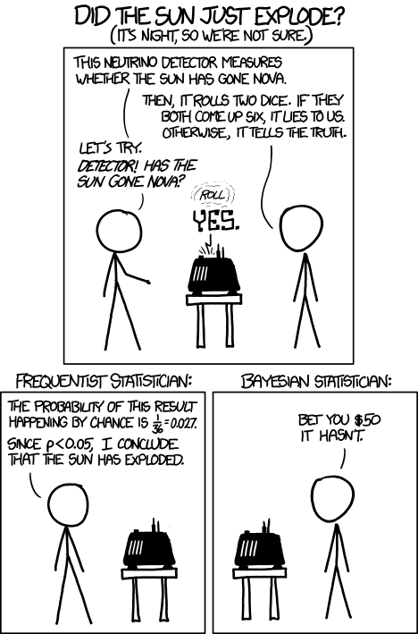
    This relates nicely to several previous posts here.

    Frequentists vs Bayesians

    Copyright © xkcd.

    Tags: , , , ,

  • Posted by Konstantin 12.02.2010 4 Comments

    Statistics is mainly about using the observed data to make conclusions about the "real state of affairs", underlying that data. A classical and most widely spread technique for making these conclusions is based on significance testing. In simple terms, the idea of significance testing is to ask the question: "if the real state of affairs were X, how probable would it be for us to obtain the data D we are currently observing?". If the answer is "rather unprobable" (e.g. p < 0.05), the common decision is to reject the proposition X in favor of the alternative "not X". Otherwise the researcher claims to "see no reason to reject X".

    The logic behind that reasoning seems quite solid from the first glance, yet it is well known to be faulty. Naturally, the fact that the likelihood of the data P(D | X) is low need not imply that the underlying hypothesis is wrong - it might very well be the case that the data by itself is already rare enough to make this value low. The only correct way of making sound judgments is to consider the a-posteriori probability of the hypothesis P(X | D) instead. However, the latter can be quite inconvenient to compute. Besides, the wild popularity of significance tests and p-values seems to indicate that the issue is not at all that serious. Really, P(X | D) looks so similar to P(D | X), who cares?

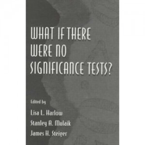
    Book cover

    The book "What If There Were No Significance Tests?", which I stumbled upon recently while browsing a stray library shelf, makes it clear that this issue is not a joke. It is a collection of chapters written by renowned statisticians (most of which some-why work in the field of psychology), that quite convincingly condemns the widespread overuse of p-values and the related significance-based hypothesis testing in favor of other approaches. The main point is nailed quite precisely in the very first essay by Jacob Cohen, which I strongly advise you to read right now in order to get rid of any illusions you might still have regarding significance testing. And when you're done with that, you can continue reading this post.

    In the following I shall provide my personal summary of the marvelous "Member of Congress" example from J.Cohen's essay. So far it is the best illustration I know of, about why exactly it is dangerous to use significance tests blindly.

    Improbable does not mean impossible

    Consider the following situation. We have observed a person which we know to be a Member of the US Congress. We are interested in testing the hypothesis, that this person is an American citizen. To apply the significance testing methodology, we proceed by estimating the p-value:

    P(Congressman | American) ~ 535/300 000 000.

    This is clearly below the popular 0.05 threshold. As a result, we are forced to reject the null-hypothesis and conclude that the person is not an American citizen. Bummer.

    What is the problem here? Well, one thing is worth noting - while the probability for an American to be a congressman is low, it is even lower (precisely, zero), for a non-American. So maybe we would have been better off if we expanded the procedure above to the following "maximum-likelihood"-style reasoning:

    Considering that the likelihood P(Congressman | American) is greater than the likelihood P(Congressman | non-American), we must conclude that the person in front of us is an American rather than not.

    Did we just solve the problem? Is it enough to consider "p-values both ways" to clear things up? No!

    Maximum likelihood does not work

    Let us now consider a reversed situation. We are faced with a person, which, we know, is an American. We are interested in the hypothesis that he is a congressman. Compute the two likelihoods:

    P(American | Congressman) = 1

    P(American | not Congressman) ~ 300 000 000 / 6 700 000 000

    Observing that the first likelihood is greater than the second we are forced to conclude that the person in front of us is indeed a congressman. Bummer, again!

    Only by multiplying the likelihood with the marginal probability P(Congressman) could we have obtained the correct decision. Which is, to say, we must have been estimating the probabilities the other way around from the start.

    To summarize, be wary of these pitfalls. I would not agree with the strong negative opinion of the authors of the book, though. After all, a lot of stuff is quite fruitfully done nowadays using p-values only. However, each time you use them, do it sensibly and keep in mind the following two aspects:

    1. If your p-value is low, can this be solely due to low marginal probability of the data? What is the "reversed" p-value? What is the power of your test?
    2. If you suspect that your hypotheses might be subject to a highly non-uniform prior probabilities, do not use bare p-values. You must consider the prior!

    Tags: , ,

  • Posted by Konstantin 28.01.2009 5 Comments

    Imagine that you have just derived a novel IQ test. You have established that for a given person the test produces a normally-distributed unbiased estimate of her IQ with variance 102. That is, if, for example, a person has true IQ=120, the test will result in a value from a N(120,102) distribution. Also, from your previous experiments you know that among all the people, IQ has a N(110,152) distribution.

    One a sunny Monday morning you went out on a street and requested the first bypasser (whose name turned out to be John) to take your test. The resulting score was t=125. The question is: what can you conclude now about the true IQ of that person (assuming, of course, that there is such a thing as a "true IQ"). There are at least two reasonable approaches to this problem.

    1. You could apply the method of maximum likelihood. Here's John, standing beside you, and you know his true IQ must be some real number a. The test produced an unbiased estimate of a equal to 125. The likelihood of the data (i.e. the probability of obtaining a test score of 125 for a given a) is therefore:

          \[P[T=125|A=a]=\frac{1}{\sqrt{2\pi 10^2}}\exp\left(-\frac{1}{2}\frac{(125-a)^2}{10^2}\right)\]

      The maximum likelihood method suggests picking the value of a that maximizes the above expression. Finding the maximum is rather easy here and it turns out to be at a=125, which is pretty natural. You thus conclude that the best what you can say about John's true IQ is that it is approximately 125.

    2. An alternative way of thinking is to use the method of maximum a-posteriori probability, where instead of maximizing likelihood P[T=125|A=a], you maximize the a-posteriori probability P[A=a|T=125]. The corresponding expression is:

       \begin{multiline} P[A=a|T=125] \sim P[T=125|A=a]\cdot P[A=a] = \\ = \frac{1}{\sqrt{2\pi 10^2}}\exp\left(-\frac{1}{2}\frac{(125-a)^2}{10^2}\right)\cdot \frac{1}{\sqrt{2\pi 15^2}}\exp\left(-\frac{1}{2}\frac{(110-a)^2}{15^2}\right) \end{multiline}

      Finding the required maximum is easy again, and the solution turns out to be a=120.38. Therefore, by this logic, John's IQ should be considered to be somewhat lower than what the test indicates.

    Which of the two approaches is better? It might seem utterly unbelievable, but the estimate provided by the second method is, in fact, closer to the truth. The straightforward "125", proposed to by the first method is biased, in the sense that on average this estimate is slightly exaggerated. Think how especially unintuitive this result is from the point of view of John himself. Clearly, his own "true IQ" is something fixed. Why on Earth should he consider "other people" and take into account the overall IQ distribution just to interpret his own result obtained from an unbiased test?

    To finally confuse things, let us say that John got unhappy with the result and returned to you to perform a second test. Although it is probably impossible to perform any real IQ test twice and get independent results, let us imagine that your test can indeed be repeated. The second test, again, resulted in a score of 125. What IQ estimate would you suggest now? On one hand, John himself came to you and this time you could regard his IQ as a "real" constant, right? But on the other hand, John is just a person randomly picked from the street, who happened to take your test twice. Go figure.

    PS: Some additional remarks are appropriate here:

    • Although I'm not a fan of The Great Frequentist-Bayesian War, I cannot but note that the answer is probably easier if John is a Bayesian at heart, because in this case it is natural for him to regard "unknown constants" as probability distributions and consider prior information in making inferences.
    • If it is hard for you to accept the logic in the presented situation (as it is for me), some reflection on the similar, but less complicated false positive paradox might help to relieve your mind.
    • In general, the correct way to obtain the true unbiased estimate is to compute the mean over the posterior distribution:

          \[E[a|T=125] = \int a \mathrm{dP}[a|T=125]\]

      In our case, however, the posterior is symmetric and therefore the mean coincides with the maximum. Computing the mean by direct integration would be much more complicated.

    Tags: , , , ,