• Posted by Konstantin 11.11.2016 4 Comments

    A question on Quora reminded me that I wanted to post this explanation here every time I got a chance to teach SVMs and Kernel methods, but I never found the time. The post expects basic knowledge of those topics from the reader.

    Introductory Background

    The concept of kernel methods is probably one of the coolest tricks in machine learning. With most machine learning research nowadays being centered around neural networks, they have gone somewhat out of fashion recently, but I suspect they will strike back one day in some way or another.

    The idea of a kernel method starts with the curious observation that if you take a dot product of two vectors, x^T y, and square it, the result can be regarded as a dot product of two "feature vectors", where the features are all pairwise products of the original inputs:

        \begin{align*} &k(x,y) = (x^Ty)^2 = (\sum_i x_iy_i)^2 = \sum_{i,j} x_ix_jy_iy_j \\ & = \langle (x_1x_1, x_1x_2,\dots,x_ix_j,\dots,x_nx_n), (y_1y_1,\dots,y_iy_j,\dots,y_ny_n)\rangle \end{align*}

    Analogously, if you raise x^Ty to the third power, you are essentially computing a dot product within a space of all possible three-way products of your inputs, and so on, without ever actually having to see those features explicitly.

    If you now take any linear model (e.g. linear regression, linear classification, PCA, etc) it turns out you can replace the "real" dot product in its formulation model with such a kernel function, and this will magically convert your model into a linear model with nonlinear features (e.g. pairwise or triple products). As those features are never explicitly computed, there is no problem if there were millions or billions of them.

    Consider, for example, plain old linear regression: f(x) = w^Tx + b. We can "kernelize" it by first representing w as a linear combination of the data points (this is called a dual representation):

        \[f(x) = \left(\sum_i \alpha_i x_i\right)^T x + b = \sum_i \alpha_i (x_i^T x) + b,\]

    and then swapping all the dot products x_i^T x with a custom kernel function:

        \[f(x) = \sum_i \alpha_i k(x_i,x) + b.\]

    If we now substitute k(x,y) = (x^T y)^2 here, our model becomes a second degree polynomial regression. If k(x,y) = (x^T y)^5 it is the fifth degree polynomial regression, etc. It's like magic, you plug in different functions and things just work.

    It turns out that there are lots of valid choices for the kernel function k, and, of course, the Gaussian function is one of these choices:

        \[k(x, y) = \exp\left(-\frac{|x - y|^2}{2\sigma^2}\right).\]

    It is not too surprising - the Gaussian function tends to pop up everywhere, after all, but it is not obvious what "implicit features" it should represent when viewed as a kernel function. Most textbooks do not seem to cover this question in sufficient detail, usually, so let me do it here.

    The Gaussian Kernel

    To see the meaning of the Gaussian kernel we need to understand the couple of ways in which any kernel functions can be combined. We saw before that raising a linear kernel to the power i makes a kernel with a feature space, which includes all i-wise products. Now let us examine what happens if we add two or more kernel functions. Consider k(x,y) = x^Ty + (x^Ty)^2, for example. It is not hard to see that it corresponds to an inner product of feature vectors of the form

        \[(x_1, x_2, \dots, x_n, \quad x_1x_1, x_1x_2,\dots,x_ix_j,\dots, x_n x_n),\]

    i.e. the concatenation of degree-1 (untransformed) features, and degree-2 (pairwise product) features.

    Multiplying a kernel function with a constant c is also meaningful. It corresponds to scaling the corresponding features by \sqrt{c}. For example, k(x,y) = 4x^Ty = (2x)^T(2y).

    Still with me? Great, now let us combine the tricks above and consider the following kernel:

        \[k(x,y) = 1 + x^Ty + \frac{(x^Ty)^2}{2} + \frac{(x^Ty)^3}{6}.\]

    Apparently, it is a kernel which corresponds to a feature mapping, which concatenates a constant feature, all original features, all pairwise products scaled down by \sqrt{2} and all triple products scaled down by \sqrt{6}.

    Looks impressive, right? Let us continue and add more members to this kernel, so that it would contain all four-wise, five-wise, and so on up to infinity-wise products of input features. We shall choose the scaling coefficients for each term carefully, so that the resulting infinite sum would resemble a familiar expression:

        \[\sum_{i=0}^\infty \frac{(x^Ty)^i}{i!} = \exp(x^Ty).\]

    We can conclude here that k(x,y) = \exp(x^Ty) is a valid kernel function, which corresponds to a feature space, which includes products of input features of any degree, up to infinity.

    But we are not done yet. Suppose that we decide to normalize the inputs before applying our linear model. That is, we want to convert each vector x to \frac{x}{|x|} before feeding it to the model. This is quite often a smart idea, which improves generalization. It turns out we can do this “data normalization” without really touching the data points themselves, but by only tuning the kernel instead.

    Consider again the linear kernel k(x,y) = x^Ty. If we normalize the vectors before taking their inner product, we get

        \[\left(\frac{x}{|x|}\right)^T\left(\frac{y}{|y|}\right) = \frac{x^Ty}{|x||y|} = \frac{k(x,y)}{\sqrt{k(x,x)k(y,y)}}.\]

    With some reflection you will see that the latter expression would normalize the features for any kernel.

    Let us see what happens if we apply this kernel normalization to the “infinite polynomial” (i.e. exponential) kernel we just derived:
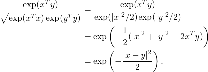
        \begin{align*} \frac{\exp(x^Ty)}{\sqrt{\exp(x^Tx)\exp(y^Ty)}} &= \frac{\exp(x^Ty)}{\exp(|x|^2/2)\exp(|y|^2/2)}  \\ &= \exp\left(-\frac{1}{2}(|x|^2+|y|^2-2x^Ty)\right) \\ &= \exp\left(-\frac{|x-y|^2}{2}\right). \end{align*}

    Voilà, the Gaussian kernel. Well, it still lacks \sigma^2 in the denominator but by now you hopefully see that adding it is equivalent to scaling the inputs by 1/\sigma

    To conclude: the Gaussian kernel is a normalized polynomial kernel of infinite degree (where feature products if i-th degree are scaled down by \sqrt{i!} before normalization). Simple, right?

    An Example

    The derivations above may look somewhat theoretic if not "magical", so let us work through a couple of numeric examples. Suppose our original vectors are one-dimensional (that is, real numbers), and let x = 1, y = 2. The value of the Gaussian kernel k(x, y) for these inputs is:

        \[k(x, y) = \exp(-0.5|1-2|^2) \approx 0.6065306597...\]

    Let us see whether we can obtain the same value as a simple dot product of normalized polynomial feature vectors of a high degree. For that, we first need to compute the corresponding unnormalized feature representation:

        \[\phi'(x) = \left(1, x, \frac{x^2}{\sqrt{2!}}, \frac{x^3}{\sqrt{3!}}, \frac{x^4}{\sqrt{4!}}, \frac{x^5}{\sqrt{5!}}\dots\right).\]

    As our inputs are rather small in magnitude, we can hope that the feature sequence quickly approaches zero, so we don't really have to work with infinite vectors. Indeed, here is how the feature sequences look like:

    ----\phi'(1) = (1, 1, 0.707, 0.408, 0.204, 0.091, 0.037, 0.014, 0.005, 0.002, 0.001, 0.000, 0.000, ...)

    ----\phi'(2) = (1, 2, 2.828, 3.266, 3.266, 2.921, 2.385, 1.803, 1.275, 0.850, 0.538, 0.324, 0.187, 0.104, 0.055, 0.029, 0.014, 0.007, 0.003, 0.002, 0.001, ...)

    Let us limit ourselves to just these first 21 features. To obtain the final Gaussian kernel feature representations \phi we just need to normalize:

    ----\phi(1) =\frac{\phi'(1)}{|\phi'(1)|} = \frac{\phi'(1)}{1.649} = (0.607, 0.607, 0.429, 0.248, 0.124, 0.055, 0.023, 0.009, 0.003, 0.001, 0.000, ...)

    ----\phi(2) =\frac{\phi'(2)}{|\phi'(2)|} = \frac{\phi'(2)}{7.389} = (0.135, 0.271, 0.383, 0.442, 0.442, 0.395, 0.323, 0.244, 0.173, 0.115, 0.073, 0.044, 0.025, 0.014, 0.008, 0.004, 0.002, 0.001, 0.000, ...)

    Finally, we compute the simple dot product of these two vectors:

        \[\scriptstyle\phi(1)^T\phi(2) = 0.607\cdot 0.135 + 0.607\cdot 0.271 + \dots = {\bf 0.6065306}602....\]

    In boldface are the decimal digits, which match the value of \exp(-0.5|1-2|^2). The discrepancy is probably more due to lack of floating-point precision rather than to our approximation.

    A 2D Example

    The one-dimensional example might have seemed somewhat too simplistic, so let us also go through a two-dimensional case. Here our unnormalized feature representation is the following:

        \begin{align*} \scriptscriptstyle\phi'(&\scriptscriptstyle x_1, x_2) = \left(1, x_1, \frac{x_1x_1}{\sqrt{2!}}, \frac{x_1x_2}{\sqrt{2!}}, \frac{x_2x_1}{\sqrt{2!}}, \frac{x_2x_2}{\sqrt{2!}}, \right. \\ &\scriptscriptstyle \left.\frac{x_1x_1x_1}{\sqrt{3!}}, \frac{x_1x_1x_2}{\sqrt{3!}}, \frac{x_1x_2x_1}{\sqrt{3!}}, \frac{x_1x_2x_2}{\sqrt{3!}}, \frac{x_2x_1x_2}{\sqrt{3!}},  \frac{x_2x_2x_1}{\sqrt{3!}}, \dots\right).\\ \end{align*}

    This looks pretty heavy, and we didn't even finish writing out the third degree products. If we wanted to continue all the way up to degree 20, we would end up with a vector with 2097151 elements!

    Note that many products are repeated, however (e.g. x_1x_2 = x_2x_1), hence these are not really all different features. Let us try to pack them more efficiently. As you'll see in a moment, this will open up a much nicer perspective on the feature vector in general.

    Basic combinatorics will tell us, that each feature of the form \frac{x_1^a x_2^b}{\sqrt{n!}} must be repeated exactly \frac{n!}{a!b!} times in our current feature vector. Thus, instead of repeating it, we could replace it with a single feature, scaled by \sqrt{\frac{n!}{a!b!}}. "Why the square root?" you might ask here. Because when combining a repeated feature we must preserve the overall vector norm. Consider a vector (v, v, v), for example. Its norm is \sqrt{v^2 + v^2 + v^2} = \sqrt{3}|v|, exactly the same as the norm of the single-element vector (\sqrt{3}v).

    As we do this scaling, each feature gets converted to a nice symmetric form:

        \[\sqrt{\frac{n!}{a!b!}}\frac{x_1^a x_2^b}{\sqrt{n!}} = \frac{x_1^a x_2^b}{\sqrt{a!b!}} = \frac{x^a}{\sqrt{a!}}\frac{x^b}{\sqrt{b!}}.\]

    This means that we can compute the 2-dimensional feature vector by first expanding each parameter into a vector of powers, like we did in the previous example, and then taking all their pairwise products. This way, if we wanted to limit ourselves with maximum degree 20, we would only have to deal with 21^2 = 231 features instead of 2097151. Nice!

    Here is a new view of the unnormalized feature vector up to degree 3:

        \[\phi'_3(x_1, x_2) = \scriptstyle\left(1, x_1, x_2, \frac{x_1^2}{\sqrt{2!}}, \frac{x_1x_2}{\sqrt{1!1!}}, \frac{x^2}{\sqrt{2!}}, \frac{x_1^3}{\sqrt{3!}}, \frac{x_1^2x_2}{\sqrt{2!1!}}, \frac{x_1x_2^2}{\sqrt{1!2!}}, \frac{x_2^3}{\sqrt{3!}}\right).\]

    Let us limit ourselves to this degree-3 example and let x = (0.7, 0.2), y = (0.1, 0.4) (if we picked larger values, we would need to expand our feature vectors to a higher degree to get a reasonable approximation of the Gaussian kernel). Now:

    ----\phi'_3(0.7, 0.2) = (1, 0.7, 0.2, 0.346, 0.140, 0.028, 0.140, 0.069, 0.020, 0.003),

    ----\phi'_3(0.1, 0.4) = (1, 0.1, 0.4, 0.007, 0.040, 0.113, 0.000, 0.003, 0.011, 0.026).

    After normalization:

    ----\phi_3(0.7, 0.2) = (0.768, 0.538, 0.154, 0.266, 0.108, 0.022, 0.108, 0.053, 0.015, 0.003),

    ----\phi_3(0.1, 0.4) = (0.919, 0.092, 0.367, 0.006, 0.037, 0.104, 0.000, 0.003, 0.010, 0.024).

    The dot product of these vectors is 0.8196\dots, what about the exact Gaussian kernel value?

        \[\exp(-0.5|x-y|^2) = 0.{\bf 81}87\dots.\]

    Close enough. Of course, this could be done for any number of dimensions, so let us conclude the post with the new observation we made:

    The features of the unnormalized d-dimensional Gaussian kernel are:

        \[\phi({\bf x})_{\bf a} = \prod_{i = 1}^d \frac{x_i^{a_i}}{\sqrt{a_i!}},\]

    where {\bf a} = (a_1, \dots, a_d) \in \mathbb{N}_0^d.

    The Gaussian kernel is just the normalized version of that, and we know that the norm to divide by is \sqrt{\exp({\bf x}^T{\bf x})}. Thus we may also state the following:

    The features of the d-dimensional Gaussian kernel are:

        \[\phi({\bf x})_{\bf a} = \exp(-0.5|{\bf x}|^2)\prod_{i = 1}^d \frac{x_i^{a_i}}{\sqrt{a_i!}},\]

    where {\bf a} = (a_1, \dots, a_d) \in \mathbb{N}_0^d.

    That's it, now you have seen the soul of the Gaussian kernel.

    Tags: , , , , , ,

  • Posted by Konstantin 18.09.2015 No Comments

    Steganography is a marvelous subject, which could be considered a subfield of cryptography. Unfortunately, it is some-why absolutely underrated nowadays. It is not covered by the standard computer science curricula (although it would fit perfectly both within lectures on Cryptography as well as Signal Processing), and way too many people believe steganography is something akin to adding grey stamps to images in Photoshop. Even the almighty Wikipedia, in its corresponding article, does not provide a decently clear view of the field, in my opinion. To fix this I thought I'd give a try at making up a short explanation myself.

    As mentioned, steganography is somewhat of a fellow discipline to cryptography. While the goal of cryptography is to protect the communication channel between Alice and Bob from some hypothetical evil Eve, the goal of steganography is to conceal the fact of communication itself. The classical setting is described as follows: Alice and Bob are kept imprisoned by the evil warden Walter. They are allowed to talk to each other, but Walter is listening to everything. How could Alice and Bob arrange a prison break without raising suspicion?

    Steganographic problems

    More specifically, steganographic problems can be divided into steganography against a passive warden, and steganography against an active warden.

    Passive warden steganography

    In this case Walter can only observe Alice and Bob's communication, but may not interfere. Walter's task is to be able to detect which of the messages between Alice and Bob contain secret meanings (if they do). If Walter comes up with a method by which he can distinguish innocent messages from the ones with a secret meaning with nontrivial probability, we shall say that Walter has succeeded in a "passive attack" on Alice and Bob's steganographic system.

    Besides helping imaginary prisoners hide from imaginary wardens, passive steganography has many practical applications. For example, some printers add a barely visible watermark to each printed page, which identifies the printer model and the date. Radio and TV advertisers sometimes include in their clips a hidden identifier of the product being advertised (which simplifies automated airtime monitoring and validation). Storage of image metainfo within the image itself (e.g. storing the patient id within its X-ray picture) may prevent confusion when data is transferred or converted, etc.

    It must be noted, that from the perspective of classical cryptography the methods mentioned above are not very interesting. Indeed, it is customary to assume in cryptography that all the details of the protocol used between Alice and Bob are open to all parties, including Walter. The only thing that Walter should not know is the "key". Without knowing this key Walter should be incapable of attacking the system. This is not the case in the examples with the printers and advertisements. No keys are involved and anyone who knows the algorithm can immediately discover the hidden message (i.e. attack the system).

    The methods for designing such systems focus primarily on techniques for adding information to a known audio/video/textual signal without distorting it in a perceivable manner and, possibly, making the presence of this information resilient to transformations that the signal may pass (video streaming, file format conversion, text normalization, etc). Consequently, the complexity of many such methods lies mostly in the area of signal processing. In the case of audio, for example, it could mean finding sound frequency components that, on one hand, will be left unchanged by most audio codecs, yet on the other hand could be modified without the listener perceiving the change. In some sense it resembles a fight between the codec (which attempts to remove any redundant channels) and the steganographic system (which aims to make use of any redundancy remaining).

    Active warden steganography

    A more interesting situation is where Walter is not only listening in to Alice and Bob's communications, but may also actively interfere, removing any potential hidden meanings. The best example here is copyright protection. They say that movies, when shown in cinemas, would usually contain a steganographic watermark in their video signal, which identifies the particular movie theatre. The "warden" here is a movie pirate, who might know about the existence of the watermark, and would be interested in removing it (without corrupting the movie itself, of course). Consequently, the watermark must be included in a way, where Walter the pirate is incapable of removing it, even if he knew all the details of the watermarking algorithm (except for a secret key, of course). Besides movie watermarking, similar techniques could be used by other authors to "sign" their creations so that their authorship could later be established, when necessary.

    Methods

    Multiple methods exist for solving both the active and passive warden steganography. Not being able to list all of them, I will mention just the two core concepts, which I think are enough for an introductory overview.

    LSB-steganography

    The most well-known example of steganography - least-significant-bit (LSB) steganography - is applicable to analog data, such as music and images. The idea is that small changes in some values (pixels, frequency components) of an analog signal would not affect the perception of the signal in a notable way. For example, by tuning some pixels in an image one could transmit several bits of additional information. Of course, the choice of those pixels should be determined using a shared secret key, otherwise Walter could easily detect or remove the covert message.

    The problem in the most naive version of this approach is that not every pixel in an image can be safely modified. For example, in regions filled with a single color any such change will be easy to spot. This can be overcome by only picking the pixels with enough variability in their neighborhood. Another weakness of the method is that the steganogram may be easy to remove by resizing or cropping the image. This can be prevented by hiding information in the spectral components rather than pixels - those are more resistant to the usual transformations. In fact, if we are dealing with a photograph or anything else that will be saved as a JPEG file, this approach would be quite nontrivial to break. The same ideas are used for steganographic processing of audio and video signals as well.

    Equivalence-class steganography

    Quite often Alice has a choice for multiple options for sending the same message. For example, when writing a text message to Bob, she can choose the phrasings. She can write "Hi" instead of "Hello", "Robert" instead of "Bob", punctuation can be used in multiple ways, and so on. When Alice is writing a novel, she is free to choose the names of the characters and places, chapter titles and even the order of events. Knowing the possible equivalence classes for the messages to be sent (e.g. words or sentences) as well as a common key, Alice may easily choose her words so that only Bob would be able to grasp whether there is a secret meaning and, if so, what it is.

    A simple practical example of a coding algorithm is the following: Alice will code a single bit by each sentence of her text. For obtaining this bit, Bob will have to apply a hash function to the sentence plus the secret key and use the last bit of that hash. During coding Alice will simply have to choose words so that each sentence would correspond to a correct bit.

    In its bare form the method is easy to attack - Walter may try to rephrase the text himself on transmission. This, in turn, can be overcome if Alice would hide the bits only into particularly chosen words or word sets (which can only be found by knowing the key), and do it using redundant coding (thus Walter would need to significantly alter the text if he wanted to be sure the message is removed). If Alice hides the message into the names of the characters of her novel, Walter may have no chances at all.

    Methods like that are claimed to be used by large software companies to watermark their code (here, instead of choosing synonymous words a specific algorithm will be choosing synonymous bytecode instructions). This makes it possible to track the particular license which was used to leak a pirated version. Another example is geographic mapping software, which may use various equivalent ways of displaying a fractal shore in order to watermark the image.

    As noted, other approaches and techniques exist (I did not find the space to properly mention public key steganography here, for example), yet I belive that LSB and EC-steganography largely illustrate the core ideas behind modern steganography in general as well as its possibilities and limitations. For those interested in the security proofs behind such techniques, this paper is a must read.


    Tags: , , ,

  • Posted by Konstantin 07.09.2015 2 Comments

    Research and engineering always go hand in hand. Their relationship is so tight that often people cease to see the difference. Indeed, both are development activities that bring along technical advances. Many researchers work in engineering companies, many engineers do what is essentially research, is there even a need to see the difference? Quite often there is. Let me highlight this difference.

    Research (sometimes synonymous with "science") is, ideally, an experimental activity, which aims to explore some space of possibilities in order to hopefully come up with a certain "understanding" of what those possibilities are or how they should be used. Researchers primarily deliver written reports, summarizing their findings. There is absolutely no guarantee that those findings would be "interesting" or "useful" to any degree - indeed, a research project by definition starts off in a position of uncertainty. As a result, for practical, commercial or investment purposes, research is always a risky activity. It may take a long time, it will produce mostly text, and there is no guarantee that the results will be of use. The upside of this risk is, of course, the chance to stumble upon unique innovation, which may eventually bring considerable benefits. Later.

    Engineering is a construction activity, where existing knowledge and tools are put together to deliver actual products. In order for this process to be successful, experimentation and uncertainty must be, ideally, brought down to a minimum. Thus, when compared to pure research, engineering projects are low risk endeavors, where the expected outputs are known in advance.

    In simple terms - researchers answer questions whilst engineers build things, and by this definition those occupations are, obviously, very different. This difference is often apparent in material fields, such as construction or electronics, where the engineers can be distinguished from the researchers by the kind of tools they would mostly hold in their hands and the places they would spend their time the most. With computational fields this visual difference does not exist - both engineers and researchers spend most of their time behind a computer screen. The tools and approaches are still different, but you won't spot this unless you are in the field. I did not know the difference between Software Engineering and Computer Science until I had the chance to try both.

    Things become even more confusing when data mining gets involved. The popularity of projects, which focus on building data-driven intelligent systems, is ever growing. As a result, more and more companies seem to be eager to embrace this magical world by hiring "data scientists" to do "data science" for them. The irony of the situation is that most of those companies are engineering businesses (e.g. software developer firms) and, as such, they would not (or at least should not) normally consider hiring anyone with the word "scientist" in the job title. Because scientists are not too famous for bringing stable income, engineers are.

    The term "data science" is a vague one, but I think it is quite succinct in that it captures the exploratory aspect that is inherent in general-purpose data analysis, as well as the current state of the art in the field. Although there are some good high level tools for a wide range of "simple" machine learning tasks nowadays, as soon as you want to try something more exotic, you are often on your own, faced with uncertainty and the need to experiment before you can even try to "build" anything. For a typical engineering company such uncertainty is not a good thing to rely upon.

    It does not mean that one cannot engineer data-driven systems nowadays, it means that in reality most of the companies, whether they know it or not, need a very particular kind of "data scientists". They need specialists with a good knowledge of simple reliable tools and are capable of applying them to various data formats. Those, who would perhaps avoid excessive experimentation in favor of simple, scalable, working solutions, even if those are somehow simplistic, suboptimal and do not employ custom-designed forty-layer convolutional networks with inception blocks, which require several months to debug and train. Those, who might not know much about concentration inequalities but would be fluent in data warehousing and streaming. There's actually a name for such people: "Data engineers".

    There is nothing novel about the use of such terminology, yet I still regularly encounter way too much misunderstanding around this topic over and over again.

    In particular, I would expect way more of the "Data engineering" curricula to appear at universities alongside the more or less standard "Data science" ones. The difference between the two would be slight, but notable - pretty much of the same order as the difference between our "Computer science" and "Software engineering" master's programmes, for example.

    Tags: , , , ,

  • Posted by Konstantin 22.03.2015 4 Comments

    This is a repost of my quora answer to the question: In layman's terms, how does Naive Bayes work?

    Suppose that you are a working as a security guard at the airport. Your task is to look at people who pass the security line and pick some of them as being worthy of a more detailed screening. Now, of course, telling whether a person is a potential criminal or not by just looking at him/her is hard, if at all possible, but you need to do something. You have been put there for some reason, after all.

    One of the simplest ways to approach the problem, mentally, is the following. You assign a "risk value" for each person. At the beginning (when you don't have any information about the person at all) you set this value to zero.

    Now you start studying various features of the person in front of you: is it a male or a female? Is it a kid? Is he behaving nervously? Is he carrying a big bag? Is he alone? Did the metal detector beep? Is he a foreigner? etc. For each of those features you know (subconsciously due to your presuppositions, or from actual statistics) the average increase or decrease in risk of the person being a criminal that it entails. For example, if you know that the proportion of males among criminals is the same as the proportion of males among non-criminals, observing that a person is male will not affect his risk value at all. If, however, there are more males among criminals (suppose the percentage is, say, 70%) than among decent people (where the proportion is around 50%), observing that a person in front of you is a male will increase the "risk level" by some amount (the value is log(70%/50%) ~ 0.3, to be precise). Then you see that a person is nervous. OK, you think, 90% of criminals are nervous, but only 50% of normal people are. This means that nervousness should entail a further risk increase (of log(0.9/0.5) ~ 0.6, to be technical again, so by now you have counted a total risk value of 0.9). Then you notice it is a kid. Wow, there is only 1% of kids among criminals, but around 10% among normal people. Therefore, the risk value change due to this observation will be negative (log(0.01/0.10) ~ -2.3, so your totals are around -1.4 by now).

    You can continue this as long as you want, including more and more features, each of which will modify your total risk value by either increasing it (if you know this particular feature is more representative of a criminal) or decreasing (if the features is more representative of a decent person). When you are done collecting the features, all is left for you is to compare the result with some threshold level. Say, if the total risk value exceeds 10, you declare the person in front of you to be potentially dangerous and take it into a detailed screening.

    The benefit of such an approach is that it is rather intuitive and simple to compute. The drawback is that it does not take the cross-play of features into account. It may very well be the case that while the feature "the person is a kid" on its own greatly reduces the risk value, and the feature "has a moustache" on its own has close to no effect, a combination of the two ("a kid with a moustache") would actually have to increase the risk by a lot. This would not happen when you simply add the separate feature contributions, as described above.

    Tags: , , , , , ,

  • Posted by Konstantin 27.01.2013 7 Comments

    Most results that are published in mathematics and natural sciences are highly technical and obscure to anyone outside the particular area of research. Consequently, most scientific publications and discoveries do not get any media attention at all. This is a problem both for the public (which would benefit from knowing a bit more about our world), the science in general (which would benefit from wider dissemination) and the scientists themselves (which would certainly appreciate if their work reached more than a couple of other people). The issue is usually addressed by the researchers trying to popularize their findings — provide simple interpretations, which could be grasped by the layman without the need to understand the foundations. Unfortunately, if the researcher was lucky to grab enough media attention, chances are high the process of "popularization" will get completely out of hands, and the message received by the public will have nothing to do with the original finding.

    There are some theorems in pure mathematics, which happened to suffer especially seriously from this phenomenon. My two most favourite examples are the Heizenberg's uncertainty principle and Gödel's incompleteness theorems. Every once in a while I stumble on pieces, written by people who have zero knowledge of basic physics (not even mentioning quantum mechanics or Fourier theory), but claim to have clearly understood the meaning and the deep implications of the uncertainty principle upon our daily lives. Even more popular are Gödel's theorems. "Science proves that some things in this world can never be understood or predicted by us, mere humans!!!" is a typical take on Gödel by the press. Oh, and it is loved by religion enthusiasts!

    This post is my desperate attempt to bring some sanity back into this world by providing a (yet another, but maybe slightly different) popular explanation for Gödel's ideas.

    Gödel's theorems explained (with enough context)

    Kurt Gödel

    Kurt Gödel

    In our daily lives we primarily use symbols to communicate and describe the world. Those may be formulas in mathematics or simply sentences in the English language. Symbol-based systems can be used in different ways. From the perspective of arts and humanities, one is welcome to construct arbitrary sequences of words and sentences, as long as the result is "beautiful", "inspiring" or "seems smart and convincing". From a more technically-minded point of view, however, one is only welcome to operate with "true and logical" statements. However, it is not at all obvious which statements should be universally considered "true and logical". There are two ways the problem can be resolved.

    Firstly, we can determine the truth by consulting "reality". For example, the phrase "All people are mortal, hence Socrates is mortal" is true because, indeed (avoiding a lecture-worth of formalities or so), in all possible universes where there are people and they are mortal, Socrates will always also be mortal.

    Secondly, we can simply postulate a set of statements, which we shall universally regard as "the true ones". To distinguish those postulated truths from the "actual truths", mentioned in the paragraph above, let us call them "logically correct statements". That is, we can hypothetically write down an (infinite) list of all the "logically correct" sentences in some hypothetical "Book of All Logically Correct Statements". From that time on, every claim not in the book will be deemed "illogical" and hence "false" (the question of whether it is false in reality would, of course, depend on the goodness and relevance of the book we created).

    This is really convenient, because now in order to check the correctness of the claim about Socrates we do not have to actually visit all the possible universes. It suffices to look it up in our book! If the book is any good, it will provide good answers, so the concept of "logical correctness" may be close or even equivalent to "actual truth". And in principle, there must exist "The Actual Book of Truth", which would list precisely the "actually true" statements.

    Unfortunately, infinite books are somewhat inconvenient to print and carry around. Luckily, we can try to represent an infinite book in a finite way using algorithms. We have all seen how a short algorithm is capable of producing an infinite amount of nonsense, haven't we? Thus, instead of looking for an (infinitely-sized) "book of truth", we should look for a (finitely-sized) "algorithm of truth", which will be either capable of generating the whole book, or checking for any given statement, whether it belongs to the book.

    Frege's propositional calculus

    Frege's propositional calculus

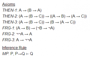
    For clarity and historical reasons,  the algorithms for describing "books of truths" are usually developed and written down using a particular "programming language", which consists of "axioms" and "inference rules". Here is one of the simplest examples of how a "program" might look like.

    This is where a natural question arises: even if we assume that we have access to "the actual book of truth", will it really be possible to compress it down to a finite algorithm? Isn't it too much to ask? It turns out it is. There is really no way to create a compact representation for any but the most trivial "books of truths".

    Besides the "asking too much" intuition, there are at least two other simple reasons why this is impossible. Firstly, most of the readers here know that there exist problems, that are in principle uncomputable. Those are usually about statements, the correctness of which cannot be checked in finite time by a finite algorithm, with the most famous example being the halting problem, as well as everything related to uncomputable numbers.

    Naturally, if we can't even use a finite algorithm to list "all truly halting programs", our hopes for getting a finite description for any more complicated "book of truths" is gone. But there is another funny reason. Once we have decided to define the book with all true statements and devise an algorithm for generating it, we must not forget to include into the book some statements about the book and the algorithm themselves. In particular, we must consider the following phrase: "This sentence will not be included in the book generated by our algorithm."

    If our algorithm does include this sentence in the generated book, the claim turns out to be false. As a result, our precious book would have false statements in it: it would be inconsistent. On the other hand, if our algorithm produces a book which does not include the above sentence, the sentence turns out to be true and the book is incomplete. It is just the liar's paradox.

    And so it is — we have to put up with the situation, where it is impossible to produce a finite representation for all true statements without stumbling into logical paradoxes. Or, alternatively, that there are mathematical statements, which cannot be checked or proven within a finite time.

    This describes what is known as "Gödel's first incompleteness theorem" (namely, the claim that in most cases our algorithm is only capable of producing either an incomplete or an inconsistent "book"). A curious corollary may be derived from it, which is known as the "Gödel's second incompleteness theorem". The theorem says that if our "book-generating algorithm" happens to include into it exactly the phrase "This book is consistent", it must necessarily be a false claim, and the algorithm must actually be inconsistent. This is often interpreted that no "honest" theory is capable of claiming it's own correctness (there are caveats, though).

    Gödel's theorems have several interesting implications for the foundations of mathematics. None the less, those are still theorems about the fundamental impossibility of using a finite algorithm for generating a book of logically correct statements without stumbling into logical paradoxes and infinite loops. Nothing more and nothing less. They have nothing to do with the experimental sciences: note how we had to cut away all connections to reality in the very first paragraphs of the explanation. And thus, Gödel's theorems are not related to the causes of "human inability to grasp the universe", "failure or success of startup business plans", or anything else of that kind.

    Tags: , , , , , ,

  • Posted by Konstantin 12.10.2011 16 Comments

    The Receiver Operating Characteristic Area Under the Curve (ROC AUC) is a measure of classifier performance, which is widely used in machine learning. Unfortunately, the obscure way the concept is explained in most sources makes it fairly hard to grasp its intuitive meaning. The name "area under the curve" itself is ill-conceived and is utterly useless in helping the intution. The aim of this post is to aid those struggling with the concept, and also present a simple and intuitive interpretation of the ROC AUC metric as the "average positive rank" which I, so far, have not seen stated explicitly elsewhere.

    To facilitate explanation, let us consider a hypothetical classification problem: classifying chocolate bars to "very good" or "just OK" (hereby we presume a chocolate bar may not be considered "bad" by definition of chocolate). Suppose we have a sample of particular chocolate bar types, for which we have carefully assigned the proper classification, e.g.:

    Item Class
    Mars 0
    Milka 1
    Kalev 0
    Lindt 1
    Ferrero-Rocher 1
    Laima 0
    Hershey's 0

    where class label "1" denotes "very good" and "0" means "just OK". Suppose we have derived a classifier which, based on some features of a chocolate bar, such as its chocolate content, packaging, country of origin, etc, attempts to assign a "goodness score" which should resemble our notion of goodness. For concreteness' sake, let us say the classifier assigned the following scores:

    Item True class Assigned score
    Milka 1 8
    Mars 0 5
    Lindt 1 3
    Ferrero-Rocher 1 3
    Kalev 0 1
    Laima 0 -3
    Hershey's 0 -5

    How do we assess the goodness of such a classifier? The "ROC approach" suggests we do the following. First, we shall plot a ROC curve. To do that, we order the chocolate bars according to their assigned score (this is already done in the table above) and use this ordering to write out the vector of the class labels (the "sorted prediction vector"):

    Highest rated item's true class Lowest rated item's true class
    1 0 1 1 0 0 0

    Obviously, the best possible classifier would order the instances so that all the ones would be on the left of all the zeroes. The particular classifier we chose here looks good, but not perfect.

    Next, we use the obtained vector to plot the ROC curve. To do this plot, forget all of the "True Positive Rate" and "False Positive Rate" nonsense you might have read about in most textbooks, and follow the following simple recipe:

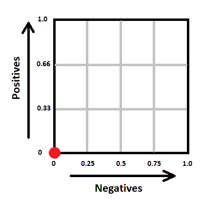
    1. Draw a square with sides of length 1. Denote its its lower left corner as the "origin", its horizontal axis as "the negatives" and its vertical axis as "the positives". Split the negatives axis in as many parts as there are examples of class "0" in the dataset. Split the positives axis in as many parts as there are examples of class "1" in your dataset. In our case, the square will look as follows:

      The ROC square

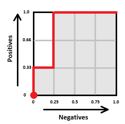
    2. Next, take the sorted prediction vector, and draw a path, starting from the origin. For each "1" in the sorted prediction vector, the path will move one step "up", and for each "0" in the vector, the path will move one step "right" (note that if you have multiple predictions with the same score, make all the corresponding "up" and "right" moves at once by drawing the corresponding diagonal). In our case, the path goes ("up", "right", "up", "up", "right", "right", "right") and hence looks as follows:

      ROC curve

    Voilà, this is your ROC curve. Obviously, the "perfect" classifier would make all the "up" steps first and the "right" steps last, hence the ideal ROC curve looks like a perfect corner. A random classifier would mix his "up" and "right" steps randomly, and the curve would most probably follow a diagonal-ish path. The one-number summary of the "goodness" of such a path is the "area under the curve" (coloured gray here), which will be 1.0 for the ideal case, and somewhere around 0.5 for the worst case. In our case the area is 10/12 ~ 0.83.

    Here comes the important question — what does this number actually mean? One good answer is given by the following probabilistic interpretation:

    The area under ROC curve specifies the probability that, when we draw one positive and one negative example at random, the decision function assigns a higher value to the positive than to the negative example.

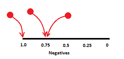
    There is, however, yet another, to my mind even more intuitive, interpretation. Define the rank of a positive example as the proportion of negative examples "to the right of it" in the sorted prediction vector. For example, if the sorted prediction vector is (1, 0, 0, 0, 0), then the rank of the sole positive item there is 1.0 (all negative examples are to the right). If the sorted prediction vector is (0, 0, 1, 0, 0), the rank is 0.5 (half of negative examples is to the right), and if the vector is (0, 0, 0, 0, 1), the rank is 0. In our chocolate bar example, the ranks of the positive examples are the following:

    Highest rated item's true class Lowest rated item's true class
    Sorted prediction vector 1 0 1 1 0 0 0
    Rank 1.0 0.75 0.75

    The "rank" thus denotes where would a classifier position a given positive item within the set of negative examples, whether closer to the "left" (rank 1) or closer to the "right" (rank 0).

    Now the average rank of all the positive examples seems like a reasonable metric of classifier performance, doesn't it? In fact, is exactly the ROC AUC! Now the value of 0.80 ROC score can be interpreted intuitively as follows: "the average positive example has about 20% of negative examples scored higher than it". This, so far, seems to me personally to be the "simplest" interpretation of the ROC AUC. So write it down:

    ROC AUC is the average positive rank.

    Tags: , ,

  • Posted by Konstantin 22.10.2008 No Comments

    A beloved child has many names, and so does the field of pattern analysis. Some people call it soft computing, others refer to it as machine learning or data-driven statistics. Although in practice all those terms denote the same approach to data analysis, there is always a certain bias hidden behind each name that relates it to its history and origins. I'm not sure whether I understand these biases correctly, but here's how I would define the terms:

    Pattern Analysis
    This is probably the most general term that refers to a kind of data analysis, where the goal is to find "something interesting" in a given dataset. We typically know what kind of things (patterns) we consider interesting (this might be an association rule, a frequent subsequence, a classifier, etc), and the task is to detect the instances of this kind of patterns. Conceptually somewhat opposite to pattern analysis would be statistical hypothesis testing, where the task is to test a given pattern for interestingness. In this sense pattern analysis is very close to the multiple hypothesis testing statistical problem.
    The simplest way to formalize this generic notion I've seen in this exposition by Tilj de Bie. Let D denote the dataset, let \Pi be the pattern space (e.g. "the space of all sequences", or "the space of all classifiers", etc), and let for each \pi\in\Pi there be a pattern function p_\pi(\cdot), so that p_\pi(D) measures the "interestingness" of this pattern with respect to the data D. Then the general task of pattern analysis is just the following maximization problem:

    \max_{\pi\in\Pi} p_\pi(D)

    Machine Learning
    Machine learning can be regarded as a specific type of pattern analysis, where the central interest lies in finding classifiers or regression functions. The dataset in this case consists of a number of "instances" x_i \in X, and the task is to find a function f: X \to Y that maps these instances to corresponding "outputs" \hat{y}_i = f(x_i) in various ways.
    In the case of supervised machine learning, a "true" output y_i is provided with each instance x_i, and the resulting function should aim to match this output for given instances (i.e. f(x_i) \approx y_i) as well as generalize to the unseen ones. Statisticians call this task regression analysis. A classical example is the problem of detecting incoming spam mail by learning the classification rule from previously labeled messages.
    The task of unsupervised machine learning is to find a classifier f without any prespecified labeling of data. Typically one searches for a function that maps similar inputs to similar outputs. If the set of outputs Y is small and discrete, the task is referred to as clustering and somewhat resembles the problem of quantization. If the outputs are continuous, the task can often be related to either factor analysis or noise reduction.
    Finally, the problem of semi-supervised machine learning is to find a classifier for a dataset where some instances have labels and some don't. This can sometimes be regarded as task of missing value imputation.
    The typical approach to all types of machine learning task usually employs the definition of a loss measure L(f), that estimates the goodness of fit for a given classifier f, and then searching for a classifier that optimizes this measure, i.e.:

    \max_f L(f)

    This defines machine learning as a certain kind of pattern analysis.

    Soft Computing
    If the previous terms denote purely mathematical approaches, for which the exact computational method of obtaining a solution is somewhat irrelevant, then this term, on the contrary, denotes a set of certain metaheuristical computational techniques for obtaining these solutions. In the narrowest sense, by soft computing one might collectively denote the areas of evolutionary algorithms, fuzzy logic and neural networks. This gives soft computing a somewhat ad-hockish flavour: "If you don't know how to solve it, simply put it into a neural network, neural networks just work".

    Data Mining
    This might be just my opinion, but I define data mining as any kind of pattern analysis, that is applied in an offline setting. Moreover, I'd say that, ideally, true data mining happens when you attempt to search for patterns in data that was not initially meant for that specific analysis, thus contradicting the classical statistical ideology "specify your hypothesis first, collect the data later".

    Knowledge Discovery from Databases
    As far as I understand it, KDD is just a YABA and marketingspeak for "data mining", somewhat in the same manner as OLAP and Business Intelligence are marketingspeak for "descriptive statistics".

    Data-Driven Statistics
    In the narrowest sense, data-driven statistics denotes all kinds of nonparametric statistical approaches. These are those methods, where one manages to perform data analysis without specifying any parameterized distributions for the inputs or the like. Typical examples would be the various resampling and randomization techniques. In the broad sense, again, this might very much be the same as pattern analysis in general.

    Any other popular terms for the same thing I've forgotten here?

    Tags: , , , , ,