• Posted by Konstantin 21.10.2019 No Comments

    Can't help sharing this lovely example, illustrating the way Python interns small integers, the lower level use of the id function as well as the power of the ctypes module.

    import ctypes
    def deref(addr, type_):
        return ctypes.cast(addr, ctypes.POINTER(type_))
    
    deref(id(29), ctypes.c_int)[4] = 100
    > 29
    100
    
    > 29*100
    10000
    
    > 25+4
    100

    Note that depending on the version of Python the value of the integer may be stored at either offset [4] or [6].

    Tags: , , , ,

  • Posted by Konstantin 22.01.2015 38 Comments

    Update from year 2017: The tool described in this post DOES NOT WORK with recent versions of Skype. Either these versions stopped saving removed messages altogether, or they are doing it in a novel manner not recognized by the tool.

    In other words - you would only recover "removed" messages if you are running older version of Skype (or these messages were sent at the time you were using that older version).

    Yesterday I happened to attend a discussion about the security and privacy of information stored locally in Skype and Thunderbird profiles. It turns out, if you obtain a person's Skype profile directory, you will be able to log in as him without the need to know the password. In addition, Dominique made a remark that Skype does not really delete the messages that are marked as "removed" in the chat window. I found that curious and decided to take a closer look.

    Indeed, there is a bunch of *.dat files in the chatsync subdirectory of the Skype's profile, which preserve all messages along with all their edits or deletions. Unfortunately, the *.dat files are in some undocumented binary format, and the only tool I found for reading those lacks in features. However, hacking up a small Python parser according to what is known about the format, along with a minimalistic GUI is a single evening's exercise, and I happened to be in the mood for some random coding.

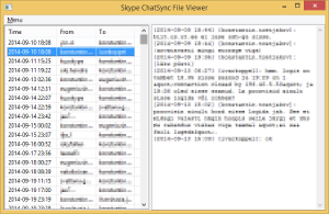
    Skype Chatsync Viewer

    Skype Chatsync Viewer

    Now, if you want to check out what was that message you or your conversation partner wrote before it was edited or deleted, this package will help. If you are not keen on installing Python packages, here is a standalone Windows executable.

    Tags: , , , , , , ,

  • Posted by Konstantin 19.06.2010 1 Comment

    The other day I was working on a Python program, which internally used a data structure for holding a set of rules. Each rule specified how some object was created from some other objects through certain procedures. The corresponding set of rules could be represented as a bunch of assignment expressions:

    # Description of the relations between objects
    some_item[1].sub_item = some_proc(other_item[2], "Text", 42)
    some_item[2].sub_item = other_proc(some_item[1], "Text", 1337)
    # ... etc

    I would manually describe the required structure using code like the following (in fact, it was slightly more complicated than that, but I hope you get the point).

    struct = Structure()
    struct.add_relation(['some_item', '[1]', '.sub_item'], 
                     ['some_proc', ['other_item', '[2]'], '"Text"', '42'])
    struct.add_relation(['some_item', '[2]', '.sub_item'],
                     ['other_proc', ['some_item', '[1]'], '"Text"', '1337'])
    now_do_something_with(struct)

    After having specified the required rules I would process them and thus solve my task, the details of which are not important here. What is important, is that all those struct.add_relation lines looked messy, long and ugly, and begged for a more concise syntax.

    One obvious choice would be to write the expressions down as strings and parse them within add_relation using ast.parse:

    struct = Structure()
    struct.add_relation(
      'some_item[1].sub_item = some_proc(other_item[2], "Text", 42)')
    struct.add_relation(
      'some_item[2].sub_item = other_proc(some_item[1], "Text", 1337)')
    now_do_something_with(struct)

    Multiple variations on this idea are possible (for example, the whole description could go in a separate configuration file), but in any case this is not a very "easy" solution.

    What I am going to show you here is that appropriate use of Python's dynamic features makes it possible to have the structure defined using Python code, side-by-side with normal Python code, in the following manner:

    @structure_definition
    def struct():
       some_item[1].sub_item = some_proc(other_item[2], "Text", 42)
       some_item[2].sub_item = other_proc(some_item[1], "Text", 1337)
    
    now_do_something_with(struct)

    This post aims to explain the mechanics behind such a solution.

    Part I: __getattr__ and __setattr__

    The first step is fairly easy. As you should know, Python is fairly flexible in that it allows you to redefine any operator, including attribute access, function invocation and assignments. We can therefore create a class StructureCreator, which does redefine all those operators as needed, and then use it in the following manner:

    s = StructureCreator()
    s.some_item[1].sub_item = s.some_proc(s.other_item[2], "Text", 42)
    s.some_item[2].sub_item = s.other_proc(s.some_item[1], "Text", 1337)

    To see what we need to do to make it work, let us explicitly write out what happens here on line 2. This line is equivalent to the following expression:

    s.__getattr__('some_item')
     .__getitem__(1)
     .__setattr__('sub_item', 
       s.__getattr__('some_proc')
        .__call__(s.__getattr__('other_item').__getitem__(2), "Text", 42)
     )

    This invocation structure neatly corresponds to the parse tree of the original expression and our StructureCreator class should therefore simply collect the information from the invocations, recursively building data structures describing the left- and right-hand sides of the expression. Finally, at the time the assignment operator __setattr__ is invoked, the collected information about the assignment can be saved appropriately. Here is an abridged conceptual example:

    class StructureBuilder:
      def __init__(self, expr=''):
        self.__dict__['__expr__'] = expr
    
      def __str__(self):
        return self.__expr__
      __repr__ = __str__
      
      def __getattr__(self, attrname):
        newname = self.__expr__ + '.' + attrname
        return StructureBuilder(newname)
    
      def __setattr__(self, attrname, val):
        newname = self.__expr__ + '.' + attrname
        print 'Saving: %s = %s' % (newname, str(val))   
    
    s = StructureBuilder()
    s.x = s.y

    It remains to implement __getitem__, __setitem__ and __call__ in a similar manner, and voila, you are all covered in syntax sugar.

    The fact that you will have to prefix all your "custom" expressions with this annoying s. might still bug your aesthetical feelings. If so, follow me to the next step.

    Part II: Hiding the Builder

    In the previous part we figured out how, by using __getattr__ and __setattr__ we can make Python interpret assignments our way. In order for it to work, however, we need to explicitly refer to an object which implements those methods, and write lines like

    s.x = s.y

    Can we somehow "hide" this object and have something analogous to automatic __getattr__ for global scope? Yes we can: Python conveniently provides us with a construction:

    exec [code] in [environment]

    which would execute our code, using the provided dictionary to resolve variables.

    Let us try it. We modify our StructureBuilder to inherit from dict and add the methods __getitem__ and __setitem__ which will happily resolve and assign to arbitrary variable names:

    class StructureBuilder(dict):
      def __init__(self, expr=''):
        self.__dict__['__expr__'] = expr
    
      def __str__(self):
        return self.__expr__
      __repr__ = __str__
      
      def __getattr__(self, attrname):
        newname = self.__expr__ + '.' + attrname
        return StructureBuilder(newname)
    
      def __setattr__(self, attrname, val):
        newname = self.__expr__ + '.' + attrname
        print 'Saving: %s = %s' % (newname, str(val))   
    
      def __getitem__(self, itemname):
        newname = self.__expr__ + '.' + str(itemname)
        return StructureBuilder(newname)
    
      def __setitem__(self, itemname, val):
        newname = self.__expr__ + '.' + str(itemname)
        print 'Saving: %s = %s' % (newname, str(val))
    

    Does it work?

    s = StructureBuilder()
    exec 'x[1].y = z' in s

    It does, but now we are providing Python code in a string, which is not at all sexy. Let us try the following instead:

    def definition():
      x[1].y = z
    
    exec definition.func_code in s

    Bummer. NameError: global name 'z' is not defined.. But why? Isn't that exactly the same as the previous attempt with a string?

    Part III: Lexical Scoping

    There is a difference in how Python compiles code in a string and in a function. To see that, let us take a look at what's inside the compiled snippets for a string

    s = 'x = y'

    and a function

    def f():
      x = y

    To do that let us use Python's bytecode disassembler module dis:

    import dis
    # First snippet (code in a string)
    dis.dis(compile(s, '', 'exec'))
    # Second snippet (code in a function)
    dis.dis(f.func_code)

    Here is the output for two snippets side by side:

    Snippet1 (String)                Snippet2 (Function)
    -------------------------------------------------------
    0 LOAD_NAME      0 (y)           0 LOAD_GLOBAL    0 (y)
    3 STORE_NAME     1 (x)           3 STORE_FAST     0 (x)
    6 LOAD_CONST     0 (None)        6 LOAD_CONST     0 (None)
    9 RETURN_VALUE                   9 RETURN_VALUE 

    Now we see it - the snippet from the string uses the LOAD_NAME and SAVE_NAME commands to access the variables, which neatly proxy the requests to our dictionary, as we want them to.

    The snippet from the function behaves in a different way. Firstly, the variable x is accessed using STORE_FAST, which is a command used for local variables. This command would not use the provided dictionary because the variable x has been determined as local to the function's scope and assigned its own memory location within the function's frame at compilation. Secondly, the variable y is accessed via LOAD_GLOBAL which, in Python's terms, refers to a variable from a surrounding lexical scope, not the dynamic scope we are trying to enforce. In short, this command also does not care about the dictionary that we provided.

    Does it mean that it is impossible to overcome the scoping rules that Python uses when compiling a function? Of course not - all we need is to modify the bytecode, replacing each LOAD_FAST, STORE_FAST, LOAD_GLOBAL and STORE_GLOBAL with LOAD_NAME and STORE_NAME.

    Part IV: Bytecode

    The required modification is well documented here, but let me give you a brief overview.
    The bytecode for a Python function f is stored in its field f.func_code.co_code. It is a sequence of bytes, which is easy to parse into opcodes. Every opcode is one byte long. Opcodes with a byte-value greater or equal than opcode.HAVE_ARGUMENT are followed by a two-byte argument. This does not seem to be well documented, but is easily read out from the code of the dis.dis function, which comes with Python. For completeness' sake, here's how a simple bytecode parser might look like:

    def bytecode(code_obj):
    	import opcode
    	code = code_obj.co_code
    	n = len(code)
    	i = 0
    	while i < n:
    		op = ord(code[i])
    		i += 1
    		oparg = None
    		if op >= opcode.HAVE_ARGUMENT:
    			oparg = ord(code[i]) + ord(code[i+1])*256
    			i += 2
    		yield (op, oparg)
    

    We now need to take the code object of our function, replace the ***_FAST and ***_GLOBAL commands with ***_NAME and create a new code object. Leaving out some details, this goes as follows:

    def as_anonymous_block(func):
      new_bytecode = []
      for (op, arg) in bytecode(func.func_code):
        if (op in [STORE_FAST, LOAD_FAST, STORE_GLOBAL, LOAD_GLOBAL]):
          new_op = LOAD_NAME or STORE_NAME, correspondingly
          new_arg = for ***_FAST we need to modify this value
          new_bytecode.append(new_op, new_arg)
        else:
          new_bytecode.append(op, arg)
      return types.CodeType( ... options, flags ... , new_bytecode)
    

    Once we perform this modification on our function object, we can use exec ... in ... to have our StructureBuilder take control of the assignments within the function:

    def definition():
      x[1].y = z
     
    exec as_anonymous_block(definition) in s
    

    Part V: Putting It All Together

    As I promised in the beginning of this post, it is possible to encapsulate the whole thing into a function annotation @structure_definition and use it as follows:

    @structure_definition
    def struct():
       some_item[1].sub_item = some_proc(other_item[2], "Text", 42)
       some_item[2].sub_item = other_proc(some_item[1], "Text", 1337)
    
    now_do_something_with(struct)

    The last step is therefore creating the @structure_definition annotation, which is rather straightforward. For a given function it processes it using as_anonymous_block, creates a new StructureBuilder object, executes the function's code in the StructureBuilder, and returns the result:

    def structure_definition(f):
      blk = as_anonymous_block(f)
      result = StructureBuilder()
      exec blk in result
      return result
    

    For further details refer to (a slightly more elaborate) example code here.

    To conclude, I should note that in my case I still ended up using the solution from Step I (i.e. the one where "dynamic" variables are prefixed with s.), because it allows to use loop variables and other constructs alongside my structure definitions much more naturally than the second method. Nonetheless, I hope you enjoyed the presented exploration as much as I did.
    Tags: , , , ,

  • Posted by Konstantin 11.10.2009 2 Comments

    I've recently stumbled upon a simple observation, which does not seem to be common knowledge and yet looks quite enlightening. Namely: polynomials provide an excellent way of modeling data in an order-agnostic manner.

    The situations when you need to represent data in an order-agnostic way are actually fairly common.  Suppose that you are given a traditional sample x_1, x_2, \dots, x_n and are faced with a task of devising a generic function of the sample, which could only depend on the values in the sample, but not on the ordering of these values. Alternatively, you might need to prove that a given statistic is constant with respect to all permutations of the sample. Finally, you might simply wish to have a convenient mapping for your feature vectors that would lose the ordering information, but nothing else.

    The most common way of addressing this problem is sorting the sample and working with the order statistics x_{(1)}, x_{(2)}, \dots, x_{(n)} instead of the original values. This is not always convenient. Firstly, the mapping of the original sample to the corresponding vector of order statistics (i.e. the sorting operation) is quite complicated to express mathematically. Secondly, the condition that the vector of order statistics is always sorted is not very pleasant to work with. A much better idea is to represent your data as a polynomial of the form

        \[p_x(z) = (z+x_1)(z+x_2)\dots(z+x_n)\,.\]

    This will immediately provide you with a marvellous tool: two polynomials p_x and p_y are equal if and only if their roots are equal, which means, in our case, that the samples x_1,\dots,x_n and y_1,\dots,y_n are equal up to a reordering.

    Now in order to actually represent the polynomial we can either directly compute its coefficients

        \[p_x(z) = z^n + a_1z^{n-1} + \dots + a_n\,,\]

    or calculate its values at any n different points (e.g. at 0,1,\dots,n-1) - in any case we end up with the same amount of data as we had originally (i.e. n values), but the new representation is order-agnostic and has, arguably, much nicer properties than the order statistics vector.

    It is not without its own problems, of course. Firstly, it requires at least \Omega(n^2) time to compute. Secondly, not every polynomial will have n real-valued roots. And thirdly, the interpretation of the new "feature vector" is not necessarily intuitive or meaningful. Yet nonetheless, it's a trick to consider.

    Tags: , , , ,

  • Posted by Konstantin 10.10.2008 4 Comments

    Note: This is a brief transcript of actions related to my recent hard disk crash recovery. I'm publishing it here in the hope it might be of use to someone someday, just as all those similar posts out there are every so often of great use to me. So if you, dear reader, are not really interested in replacing a hard disk of your DELL PC, you better save your time and skip to the next post.

    A pair of days ago I accidentally managed to test what happens if you throw a running 3-year-old DELL XPS M1210 laptop from a height of about 1.3 meters against solid floor. The result, fortunately, was radically different from what one might expect after observing that painful inelastic crash. After switching the screen off for a period of 5 seconds or so (the reasons behind this behavior being a complete mystery for me) the laptop happily resumed as if nothing had happened. A later examination revealed that the only part that was damaged was the hard disk where a number of files became unreadable.

    I presumed that it must have been the result of a strong head crash. Common knowledge suggests that a head-crashed hard disk should better be replaced, even if it continues functioning. This is because new head crashes are much more probable after the first one has happened. Thus, I went to the shop and got myself a new average-grade 160Gb SATA hard disk (these are surprisingly cheap nowadays, btw). I also bought a small external case to put my old drive into, so that I could continue using it as an external storage medium.

    In principle, the whole procedure could have ended here: I could have taken the old hard disk out, put the new one in, installed the OS onto the new disk from a CD and copied my files from the old disk with the help of the external case. However, there was one thing I didn't like about this approach. If I were to restart with a blank OS, I'd have to bother installing the proper drivers as well as several pieces of software that were shipped with the factory preinstallation of Windows XP (in particular, that enormously useless yet really impressive Logitech Video Effects webcam feature). I knew, however, that there was a way to restore the disk to the factory setting so I went on to figure out how to do it for a new hard disk. In hindsight, the whole procedure is actually rather straightforward, at least if you appreciate the virtues of the dd command.

    DELL System Restore Partition

    It seems that most DELL laptops nowadays come with a "DELL System Restore" feature, which means that there is a hidden partition on the hard disk that stores the factory-installed Ghost image of the system drive. If at boot time you press Ctrl+F11, you get the opportunity to write this image to disk thus destroying all your data but bringing the computer to its retail state.

    The hidden partition is labeled DellRestore and besides the image file it contains a bootable DOS operating system (yes, real DOS!), the program for restoring the Ghost image (restore.exe) and an autoexec.bat script that invokes this program on boot. So, if I'm not mistaken, by pressing Ctrl+F11 you just direct the laptop to boot the DellRestore partition.

    In theory, if you mirror the partition structure of your old hard drive on the new one and copy the data of the DellRestore partition, it should be possible to simply put in the new drive and press Ctrl+F11 for a proper restoration. However, my new drive was larger in capacity than the old one so I didn't want to mirror the partition structure exactly and I ended up with a somewhat more complicated procedure. The following is an approximate list of steps I went through. Don't try repeating them unless you really understand everything, though. You are also strongly advised to visit this site first.

    The Walkthrough

    1. I needed two bootable CDs here: one Knoppix Live CD and one DOS bootable CD.
    2. First, keep the old (damaged) hard disk in the laptop, put the new disk into the external case, but don't plug it in yet.
    3. Boot the Knoppix CD, when it starts switch to the command line (Ctrl+Alt+F1)
    4. Ensure that the laptop's hard disk is seen as /dev/sda and examine its partition table:
      # cfdisk /dev/sda
    5. It should have 3 partitions: DellUtility (sda1), the main NTFS partition (sda2) and DellRestore (sda3). Write down their sizes and quit cfdisk.
    6. Plug in the new disk (the one in the external case) into the USB port. Ensure that OS detects it: type
      # dmesg
      and examine the output.
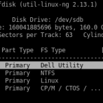
    7. Partition Table on the New Disk

      New Drive's Partition Table

      Type
      # cfdisk /dev/sdb
      and create a partition table for the new disk that mimics the one of the old one. In my case I created the first DellUtility partition of the same size and type as was sda1. I then added one NTFS partition (for the main Windows OS) and a small Linux partition (just for fun) choosing the sizes of both to my liking. Finally the fourth partition was created of the same size and type as sda3. See Figure.

    8. Copy the data of sda1 to sdb1 and sda3 to sdb4.
      # dd if=/dev/sda1 of=/dev/sdb1 bs=1024
      # dd if=/dev/sda3 of=/dev/sdb4 bs=1024
    9. Copy the master boot record of the old drive to the new one.
      # dd if=/dev/sda of=/dev/sdb bs=446 count=1
    10. Now, shutdown Knoppix
      # shutdown -h now
      remove the old disk from the laptop, take the new disk from the case and put it into the laptop. Now boot the DOS CD.
    11. When in DOS, go to disk C: (this is the DellRestore partition) subdirectory bat\:
      > cd c:\bat
    12. Execute restore.bat
      > restore.bat
      This should initiate the restore process and write the factory image to your second partition.
    13. After the restore process completed I somewhy still had the problem that the system would not boot. I booted Knoppix, opened the partition table (cfdisk /dev/sda) and discovered that the bootable flag of the second partition was gone after the restoration process. Making the partition bootable again and restarting fixed the problem.

    That's it.

    Tags: , ,