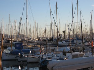
The yachts parked in the port of Palma de Mallorca might very well outnumber the presumably plentiful palm trees in this city. The photo below depicts just a small piece of the 3 kilometer-long marina, stretched along the Paseo Maritimo coastline.
For the fun of it, let's try counting the yachts on this photo. Even though it is perhaps one of the most useless exercises one might come up with, I find it amusing and not without a relation to a variety of more serious applications. Naturally, no sane computer scientist would attempt to do the counting manually when he can let a computer do this job for him. Therefore, we'll use a chance here to exploit the fantastic Scilab Image Processing toolbox.
Preprocessing
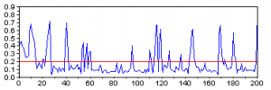
If we only want to know the number of masts, we don't need the whole image, a single line of the image that crosses all of the masts would suffice. Some pixels of this line will correspond to the sky — a brief examination shows that the RGB colour of these pixels is approximately (0.78, 0.78, 0.78). The remaining pixels will be the masts and the ropes. For each pixel, we can compute how similar this pixel's colour is to the colour of the sky (the simple euclidean distance will do OK), and thus we shall end up with a single vector, the peaks in which will correspond to the masts we need to count.
  // Read image
  img = imread("yachts.jpg");

  // Get the proper line
  img_line = img(505,:,:);

  // Subtract sky colour
  img_line = sqrt(sum((img_line - 0.78*ones(img_line)).^2, 3));
Let us now do the counting.
1. Geometric approach
A look on the picture above will tell you that a threshold of about 0.2 might be good for discriminating the masts from the background. Once we apply it, there are at least two easy ways to derive the number of masts.
- Firstly, we could count the number of pixels over the threshold and divide it by four, which seems like roughly the average width of a mast.
answer = sum(img_line > 0.2)/4
The result is ~135.
- Secondly, we could count the number of times the pixel value crosses the 0.2 boundary:
answer = sum(img_line(2:$) > 0.2 & img_line(1:($-1)) <= 0.2);
Here the result will be 158.
2. Spectral approach
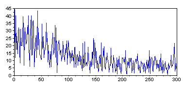
The discrete Fourier transform of a vector is a natural way for counting repeating peaks in the signal.
  ff = abs(fft(center(img_line)));
  plot(0:300, ff(1:301));
The interpretation of the resulting figure should, in theory, be simple. If the photo only contained n uniformly distributed masts, the spectrum would have one clear peak at n. In our case, unfortunately, things do not seem to be as easy. With some wishful thinking one might see major peaks around 50, 150 and 300. Now taking the previous results into consideration let us presume that 150 is the correct peak. Then 50 could correspond to the 50 "larger" masts on the image, and 300, perhaps, to the ropes.
3. Statistical approach
The original image is 1600 pixels wide. If the photo contained n masts, distributed uniformly along its width, a randomly chosen 32-pixel region would contain about n/50 masts on average. Therefore, let us select some of these random regions and count the number of masts in them manually. After multiplying the resulting numbers by 50 we should obtain estimates of the total number of masts.
  xbasc();
  rand("seed", 1);
  for i=1:9
    m = floor(rand()*(1600-32))+1;
    subplot(3,3,i);
    imshow(img([474:566], [m:(m+32)],:))
  end
Here are the estimates I got here: 200, 50, 50, 150, 150, 100, 100, 100, 100. The average comes at 111 with a standard deviation of about 50.
Summary
There are serious discrepances among the results produced by various approaches. However, if you attempt to count the masts manually, you will quickly discover that there is indeed an inherent degree of uncertainty in the number of visible masts, with the true number lying somewhere between 100 and 150. Consequently, the considered approaches to mast counting were not too far off, after all.


