Four Years Remaining

This post presumes you are familiar with PCA.

Consider the following experiment. First we generate a random vector (signal) as a sequence of random 5-element repeats. That is, something like

(0.5, 0.5, 0.5, 0.5, 0.5,   0.9, 0.9, 0,9, 0.9, 0,9,   0.2, 0.2, 0.2, 0.2, 0.2,   ... etc ... )

In R we could generate it like that:

num_steps = 50
step_length = 5;
initial_vector = c();
for (i in 1:num_steps) {
  initial_vector = c(initial_vector, rep(runif(1), step_length));
}

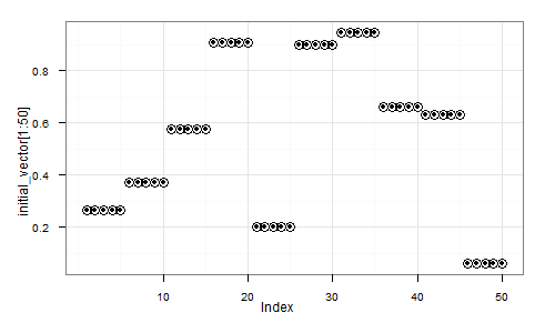
Here's a visual depiction of a possible resulting vector:

plot(initial_vector), zoomed in

Next, we shall create a dataset, where each element will be a randomly shifted copy of this vector:

library(magic) # Necessary for the shift() function
dataset = c()
for (i in 1:1000) {
  shift_by = floor(runif(1)*num_steps*step_length) # Pick a random shift
  new_instance = shift(initial_vector, shift_by)   # Generate a shifted instance
  dataset = rbind(dataset, new_instance);          # Append to data
}

Finally, let's apply Principal Component Analysis to this dataset:

pca = prcomp(dataset)

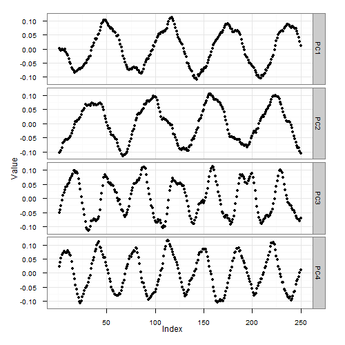
Question - how do the top principal components look like? Guess first, then read below for the correct answer.

Interestingly, the major principal components are all pretty much sine- and cosine waves

First four principal components of the "shifts" dataset

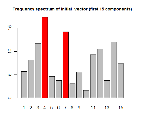
Moreover, the wave frequencies of the top-scoring principal components (4 and 7 cycles per signal in the example above) correspond exactly to the largest components of the Fourier transform of the initial signal. Observe:

fourier = fft(initial_vector)
barplot(abs(fourier)[2:16])

fft(initial_vector)

The observation bears some practical importance. Datasets that contain many "shifted copies" of otherwise similar signals are not impossible to come by. You will see those if you are studying sets of time series, which all mainly differ by the "starting time" of some event. Applying PCA to such a dataset will almost certainly result in the extraction of sinewaves, which is a variant of spectral decomposition.

Why does it work this way? I'll leave it for you to wonder. Hint - it has something to do with eigensignals of linear time-invariant systems.