Every student of computer science, who has managed to keep even a tiny shred of attention at their algorithms course, should know that sorting  numbers is a task that requires at least
  time in general. There are some special cases, such as sorting small integers, where you can use counting sort or radix sort to beat this baseline, but as long as your numbers are hypothetically arbitrarily large, you are stuck with the lower bound. Right?
Well, not really. One thing that many algorithms courses tend to skim over rather briefly is the discussion of the choice of the computation model, under which the algorithm of interest is supposed to run. In particular, the bound for sorting holds for the comparison-only model of computation — the abstract situation where the algorithm may only perform pairwise comparisons of the numbers to be sorted. No arithmetic, bit-shifts or anything else your typical processor is normally trained to do is allowed. This is, obviously, not a very realistic model for a modern computer.
Let us thus consider a different computation model instead, which allows our computer to perform any of the basic arithmetic or bitwise operations on numbers in constant time. In addition, to be especially abstract, let us also assume that our computer is capable of handling numbers of arbitrary size. This is the so-called unit-cost RAM model.
It turns out that in this case one can sort arbitrarily large numbers in linear time. The method for achieving this (presented in the work of W. Paul and J. Simon, not to be confused with Paul Simon) is completely impractical, yet quite insightful and amusing (in the geeky sense). Let me illustrate it here.
Paul-and-Simon Sorting
The easiest way to show an algorithm is to step it through an example. Let us therefore consider the example task of sorting the following array of three numbers:
a = [5, 3, 9]
Representing the same numbers in binary:
[101, 11, 1001]
Our algorithm starts with a linear pass to find the bit-width of the largest number in the array. In our case the largest number is 9 and has 4 bits:
bits = max([ceil(log2(x)) for x in a])     # bits = 4
n = len(a)                                 # n = 3
Next the algorithm will create a  -bit number
 A of the following binary form:
1 {5} 1 {5} 1 {5} 1 {3} 1 {3} 1 {3} 1 {9} 1 {9} 1 {9}
where {9}, {3} and {5} denote the 4-bit representations of the corresponding numbers. In simple terms, we need to pack each array element repeated times together into a single number. It can be computed in linear time using, for example, the following code:
temp, A = 0, 0
for x in a:
    temp = (temp<<(n*(bits+1))) + (1<<bits) + x
for i in range(n):
    A = (A<<(bits+1)) + temp
The result is 23834505373497, namely:
101011010110101100111001110011110011100111001
Next, we need to compute another 45-bit number B, which will also pack all the elements of the array times, however this time they will be separated by 0-bits and interleaved as follows:
0 {5} 0 {3} 0 {9} 0 {5} 0 {3} 0 {9} 0 {5} 0 {3} 0 {9}
This again can be done in linear time:
temp, B = 0, 0
for x in a:
    temp = (temp<<(bits+1)) + x
for i in range(n):
    B = (B<<(n*(bits+1))) + temp
The result is 5610472248425, namely:
001010001101001001010001101001001010001101001
Finally, here comes the magic trick: we subtract B from A. Observe how with this single operation we now actually perform all pairwise subtractions of the numbers in the array:
A = 1 {5} 1 {5} 1 {5} 1 {3} 1 {3} 1 {3} 1 {9} 1 {9} 1 {9}
B = 0 {5} 0 {3} 0 {9} 0 {5} 0 {3} 0 {9} 0 {5} 0 {3} 0 {9}
Consider what happens to the bits separating all the pairs. If the number on top is greater or equal to the number on the bottom of the pair, the corresponding separating bit on the left will not be carried in the subtraction, and the corresponding bit of the result will be 1. However, whenever the number on the top is less than the number on the bottom, the resulting bit will be zeroed out due to carrying:
A   = 1 {5} 1 {5} 1 { 5} 1 { 3} 1 {3} 1 { 3} 1 {9} 1 {9} 1 {9}
B   = 0 {5} 0 {3} 0 { 9} 0 { 5} 0 {3} 0 { 9} 0 {5} 0 {3} 0 {9}
A-B = 1 {0} 1 {2} 0 {12} 0 {14} 1 {0} 0 {10} 1 {4} 1 {6} 1 {0}
The same in binary (highlighted groups correspond to repetitions of the original array elements in the number A):
A   = 1 0101 1 0101 1 0101|1 0011 1 0011 1 0011|1 1001 1 1001 1 1001
B   = 0 0101 0 0011 0 1001|0 0101 0 0011 0 1001|0 0101 0 0011 0 1001
A-B = 1 0000 1 0010 0 1100|0 1110 1 0000 0 1010|1 0100 1 0110 1 0000
Each "separator" bit of A-B is effectively the result of a comparison of every array element with every other. Let us now extract these bits using a bitwise AND and sum them within each group. It takes another couple of linear passes:
x = A-B >> bits
mask, result = 0, 0
for i in range(n):
    mask = (mask<<(n*(bits+1))) + 1
for i in range(n):
    result += x & mask
    x = x >> (bits+1)
The result is now the following number:
result = 10|000000000000001|000000000000011
It is a packed binary representation of the array r = [2, 1, 3]. The number 2 here tells us that there are two elements in a, which are less or equal than a[0]=5. Similarly, the number 1 says that there is only one element less or equal than a[1]=3, and the number 3 means there are three elements less or equal than a[2]=9. In other words, this is an array of ranks, which tells us how the original array elements should be rearranged into sorted order:
r = [result >> (n*(bits+1)*(n-i-1)) & ((1<<(n*(bits+1)))-1)
                                          for i in range(n)]
a_sorted = [None]*n
for i in range(n):
    a_sorted[r[i]-1] = a[i]
And voilà, the sorted array! As presented above, the method would only work for arrays consisting of distinct non-negative integers. However, with some modifications it can be adapted to arbitrary arrays of integers or floats. This is left as an exercise to the reader.
The General Implications
There are several things one can learn from the "Paul-and-Simon sort". Firstly, it shows the immense power of the unit-cost RAM computational model. By packing arbitrary amounts of data into a single register of unlimited size, we may force our imaginary computer to perform enormously complex parallel computations in a single step. Indeed, it is known that PSPACE-complete problems can be solved in polynomial time in the unlimited-precision RAM model. This, however, assumes that the machine can do arbitrary arithmetic operations. If you limit it to only additions, subtractions and multiplications (but not divisions or bit-shifts), you still cannot sort integers faster than even using infinitely-sized registers (this is the main result of the Paul and Simon's article that inspired this post). Not obvious, is it?
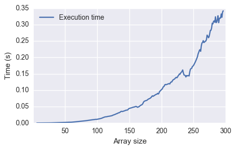
Of course, real computers can usually only perform constant-time operations on registers of a fixed size. This is formalized in the  -bit word-RAM model, and in this model the "Paul and Simon sort" degrades from a
  into a
  algorithm (with
  memory consumption). This is a nice illustration of how the same algorithm can have different complexity based on the chosen execution model.
The third thing that the "Paul and Simon sort" highlights very clearly is the power of arithmetic operations on packed values and bitstrings. In fact, this idea has been applied to derive practically usable integer sorting algorithms with nearly-linear complexity. The latter paper by Han & Thorup expresses the idea quite well:
In case you need the full code of the step-by-step explanation presented above, here it is.


