Four Years Remaining

The Secrets of Spring Motion

Posted by Konstantin 17.11.2016 3 Comments

Imagine a weight hanging on a spring. Let us pull the weight a bit and release it into motion. What will its motion look like? If you remember some of your high-school physics, you should probably answer that the resulting motion is a simple harmonic oscillation, best described by a sinewave. Although this is a fair answer, it actually misses an interesting property of real-life springs. A property most people don't think much about, because it goes a bit beyond the high school curriculum. This property is best illustrated by

The Slinky Drop

The "slinky drop" is a fun little experiment which has got its share of internet fame.

The Slinky Drop

When the top end of a suspended slinky is released, the bottom seems to patiently wait for the top to arrive before starting to fall as well. This looks rather unexpected. After all, we know that things fall down according to a parabola, and we know that springs collapse according to a sinewave, however neither of the two rules seem to apply here. If you browse around, you will see lots of awesome videos demonstrating or explaining this effect. There are news articles, forum discussions, blog posts and even research papers dedicated to the magical slinky. However, most of them are either too sketchy or too complex, and none seem to mention the important general implications, so let me give a shot at another explanation here.

The Slinky Drop Explained Once More

Let us start with the classical, "high school" model of a spring. The spring has some length $L$ in the relaxed state, and if we stretch it, making it longer by $\Delta L$ , the two ends of the spring exert a contracting force of $k\Delta L$ . Assume we hold the top of the spring at the vertical coordinate $y_{\mathrm{top}}=0$ and have it balance out. The lower end will then position at the coordinate $y_{\mathrm{bot}} = -(L+mg/k)$ , where the gravity force $mg$ is balanced out exactly by the spring force.

How would the two ends of the spring behave if we let go off the top now? Here's how:

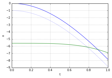
The horozontal axis here denotes the time, the vertical axis - is the vertical position. The blue curve is the trajectory of the top end of the spring, the green curve - trajectory of the bottom end. The dotted blue line is offset from the blue line by exactly $L$ - the length of the spring in relaxed state.

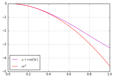
Observe that the lower end (the green curve), similarly to the slinky, "waits" for quite a long time for the top to approach before starting to move with discernible velocity. Why is it the case? The trajectory of the lower point can be decomposed in two separate movements. Firstly, the point is trying to fall down due to gravity, following a parabola. Secondly, the point is being affected by string tension and thus follows a cosine trajectory. Here's how the two trajectories look like separately:

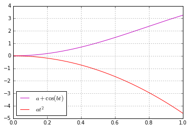
They are surprisingly similar at the start, aren't they? And indeed, the cosine function does resemble a parabola up to $o(x^3)$ . Recall the corresponding Taylor expansion:

$\cos(x) = 1 - \frac{x^2}{2} + \frac{x^4}{24} + \dots \approx 1 - \frac{x^2}{2}.$

If we align the two curves above, we can see how well they match up at the beginning:

Consequently, the two forces happen to "cancel" each other long enough to leave an impression that the lower end "waits" for the upper for some time. This effect is, however, much more pronounced in the slinky. Why so?

Because, of course, a single spring is not a good model for the slinky. It is more correct to regard a slinky as a chain of strings. Observe what happens if we model the slinky as a chain of just three simple springs:

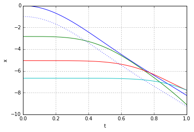
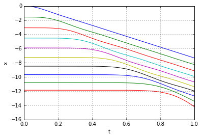
Each curve here is the trajectory of one of the nodes inbetween the three individual springs. We can see that the top two curves behave just like a single spring did - the green node waits a bit for the blue and then starts moving. The red one, however, has to wait longer, until the green node moves sufficiently far away. The bottom, in turn, will only start moving observably when the red node approaches it close enough, which means it has to wait even longer yet - by that time the top has already arrived. If we consider a more detailed model, the movement of a slinky composed of, say, 9 basic springs, the effect of intermediate nodes "waiting" becomes even more pronounced:

To make a "mathematically perfect" model of a slinky we have to go to the limit of having infinitely many infinitely small springs. Let's briefly take a look at how that solution looks like.

The Continuous Slinky

Let $x$ denote the coordinate of a point on a "relaxed" slinky. For example, in the two discrete models above the slinky had 4 and 10 points, numbered $1,\dots, 4$ and $1,\dots, 10$ respectively. The continuous slinky will have infinitely many points numbered $[0,1]$ .

Let $h(x,t)$ denote the vertical coordinate of a point $x$ at time $t$ . The acceleration of point $x$ at time $t$ is then, by definition $\frac{\partial^2 h(x,t)}{\partial^2 t}$ , and there are two components affecting it: the gravitational pull $-g$ and the force of the spring.

The spring force acting on a point $x$ is proportional to the stretch of the spring at that point $\frac{\partial h(x,t)}{\partial x}$ . As each point is affected by the stretch from above and below, we have to consider a difference of the "top" and "bottom" stretches, which is thus the derivative of the stretch, i.e. $\frac{\partial^2 h(x,t)}{\partial^2 x}$ . Consequently, the dynamics of the slinky can be described by the equation:

$\frac{\partial^2 h(x,t)}{\partial^2 t} = a\frac{\partial^2 h(x,t)}{\partial^2 x} - g.$

where $a$ is some positive constant. Let us denote the second derivatives by $h_{tt}$ and $h_{xx}$ , replace $a$ with $v^2$ and rearrange to get:

(1) $h_{tt} - v^2 h_{xx} = -g,$

which is known as the wave equation. The name stems from the fact that solutions to this equation always resemble "waves" propagating at a constant speed $v$ through some medium. In our case the medium will be the slinky itself. Now it becomes apparent that, indeed, the lower end of the slinky should not move before the wave of disturbance, unleashed by releasing the top end, reaches it. Most of the explanations of the slinky drop seem to refer to that fact. However when it is stated alone, without the wave-equation-model context, it is at best a rather incomplete explanation.

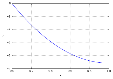
Given how famous the equation is, it is not too hard to solve it. We'll need to do it twice - first to find the initial configuration of a suspended slinky, then to compute its dynamics when the top is released.

In the beginning the slinky must satisfy $h_t(x, t) = 0$ (because it is not moving at all), $h(0, t) = 0$ (because the top end is located at coordinate 0), and $h_x(1, t) = 0$ (because there is no stretch at the bottom). Combining this with (1) and searching for a polynomial solution, we get:

$h(x, t) = h_0(x) = \frac{g}{2v^2}x(x-2).$

Next, we release the slinky, hence the conditions $h_t(x,t)=0$ and $h(0,t)=0$ disappear and we may use the d'Alembert's formula with reflected boundaries to get the solution:

$h(x,t) = \frac{1}{2}(\phi(x-vt) + \phi(x+vt)) - \frac{gt^2}{2},$

$\text{ where }\phi(x) = h_0(\mathrm{mod}(x, 2)).$

Here's how the solution looks like visually:

Notice how the part of the slinky to which the wave has not arrived yet, stays completely fixed in place. Here are the trajectories of 4 equally-spaced points on the slinky:

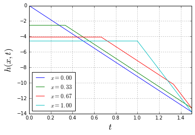
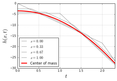
Note how, quite surprisingly, all points of the slinky are actually moving with a constant speed, changing it abruptly at certain moments. Somewhat magically, the mean of all these piecewise-linear trajectories (i.e. the trajectory of the center of mass of the slinky) is still a smooth parabola, just as it should be:

The Secret of Spring Motion

Now let us come back to where we started. Imagine a weight on a spring. What will its motion be like? Obviously, any real-life spring is, just like the slinky, best modeled not as a Hooke's simple spring, but rather via the wave equation. Which means that when you let go off the weight, the weight will send a deformation wave, which will move along the spring back and forth, affecting the pure sinewave movement you might be expecting from the simple Hooke's law. Watch closely:

Here is how the movement of the individual nodes looks like:

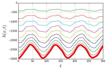
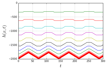
The fat red line is the trajectory of the weight, and it is certainly not a sinewave. It is a curve inbetween the piecewise-linear "sawtooth" (which is the limit case when the weight is zero) and the true sinusoid (which is the limit case when the mass of the spring is zero). Here's how the zero-weight case looks like:

And this is the other extreme - the massless spring:

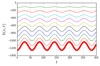
These observations can be summarized into the following obviously-sounding conclusion: the basic Hooke's law applies exactly only to the the massless spring. Any real spring has a mass and thus forms an oscillation wave traveling back and forth along its length, which will interfere with the weight's simple harmonic oscillation, making it "less simple and harmonic". Luckily, if the mass of the weight is large enough, this interference is negligible.

And that is, in my opinion, one of the interesting, yet often overlooked aspects of spring motion.

Tags: Explanation, Mathematics, Paradox, Physics, Science, Theory, Visualization