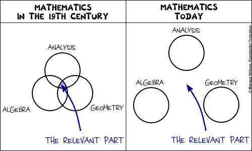
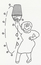
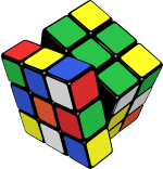
A cute joke by Margus from the recent EWSCS09 Crapcon session.
-
Tags: Comic, Fun, Humor, Mathematics, Philosophy
-
Symbols and Reality
Mathematics is a language. An abstract set of generic symbols for describing concepts, objects and systems. Take, for example, the symbol "5", "five". What is it? Is it a real-world object? No. It is just a symbol. You are free to attach to it any interpretation that you deem appropriate. Of course, most of the times you would use the common interpretation of "5" as a natural number, denoting, well, "five of something". Literally meaning that you can count something as "this, this, this, this and this".
Take a moment to reflect on the degree of generality of this simple concept, "five". It can be applied to practically anything. Five apples, five centimeters, five centuries are notions as different from each other as you could imagine, and yet all of them relate to the concept "five". On the other hand, it is not too generic to be useless: "five" is radically different from "six", "seven", and an infinity of other numbers. This kind of magical balance between generality and specificity is common to mathematics. This is what makes mathematics both widely applicable and yet still incredibly useful.
Besides just giving us symbols like 5 or 6, mathematics provides an endless variety of ways for expressing "rules", "operations", "statements", "derivations", "computations" and the like, such as 5+5=10, or
 , etc. Once again, all of these rules, operations and statements need not necessarily bear any relation with reality. After all, they all are just a cunning play with symbols. And yet, quite often they do describe reality incredibly well. I know that 512 apples and 512 apples will make 1024 apples together. How do I know it? Certainly not because I checked it on real apples! I just believe that the real-world operation of "adding apples" can be satisfactory modeled using the formal symbolic framework of natural numbers and the operation of addition on them. Why do I believe it? This is a tricky philosophical question that we shall leave aside for now. But remember that any application of mathematics to the real world is always based on a belief that the chosen model describes the world well.
The Nature of Uncertainty
There are often cases where we would like to use mathematics to model "uncertainty". Now remember that from the point of view of pure math there are no such things as inherent "certainty" and "uncertainty". Mathematics will always operate on symbols and use precise, uniquely reproducible transformation rules between these symbols. Yet there are often cases when we, in our interpretations of these symbols, would like refer to certain entities as "uncertain". The reasons can be various:
- Sometimes, we would like to use a single generalized concept to summarize multiple objects.
- What is the height of a human?
There is no single clear answer and yet it is possible to provide one using an uncertainty model such as a probability distribution. - Sometimes, we want to reason about some single numeric value which, even if it were well-defined, we just could not compute exactly.
- What is the AVERAGE height of a human?
In theory, it is a number you could measure by lining up all the people in the world and computing their average, but it is certainly an infeasible project. - Sometimes, the notion we would like to reason about is inherently not well-defined.
- What is MY height, after all?
The answer depends on a number of factors such as time, measuring equipment, my precise posture, etc. Instead of taking all of these into consideration, we prefer to exploit an uncertainty model. - Sometimes we just need a single concept to encapsulate a state of knowledge more sophisticated than pure numeric equality. For example, to express the fact like "my height IS GREATER THAN 150cm" without using the "greater than" operation.
There are also other situations, which are difficult to classify, but in all cases the idea is the same — for one reason or another we "don't know" (or "don't specify") the exact single quantity we want to reason about, an yet we still "know something" about it. In fact, amusingly, the amount of information that we use to represent an "uncertain" quantity is often much greater than the amount of information we would need to represent a "certain" one. For example, there are much more probability distributions than there are real numbers. Therefore, picking one probability distribution to represent our knowledge of a number is, in principle, a more informative step than picking a single real number. And yet, we call the former case "uncertainty" and the latter one "certainty". Because that's how we choose to name and interpret things, that's how we believe these concepts relate to reality.
Models of Uncertainty
The adjective "uncertain" is something you could, in theory, apply generically to any type of data. In a computer scientist's terms, it makes perfect sense to talk about datatypes "
uncertain int", "uncertain real", "uncertain boolean", "uncertain string", "uncertain graph", "uncertain map" and maybe even "uncertain uncertain real" and the like. Let's limit ourselves here to the consideration of uncertain numbers only, as these are the most commonly used and well-studied types of uncertainty. So how do you model (or, say, "implement") "uncertain real"? Here is a short list of the most popular options:- Approximate numbers.Although you might not consider it as a smart approach, this is probably the most common choice in practice — using a usual number to represent an uncertain one. In this case the uncertainty is purely interpretative: instead of stating
 you would, perhaps, write
  , denoting your state of ignorance. Quite often you would not even care to use the approximate equality sign, presuming it is clear from the context that you are not supposed to provide an ideally exact measurement: — What is your height? — It is 180cm. This works quite well in simple real-life situations, such as buying a kilogram of apples or discussing the horsepowers in a friend's motorbike, but is also applicable to some more technical cases, such as computing the distance to the nearest star.The advantage of such implied uncertainty is that you do not really need to deal with it. All of your familiar arithmetic operations come for free, together with their well established interpretations and the nice properties, theories and theorems. The disadvantage is that once your data is approximate, all of these theories and theorems become approximate too. So, although it could often be acceptable to claim
  , you would have problems explaining more complicated steps, such as "
 for a continuous f".But what to do if you need to perform such steps? Consider intervals instead!
 - Intervals.The second most popular method of representing an uncertain real number is to provide an interval where it falls into. It is ubiquitous in engineering disciplines. Most often an interval is expressed either as
 or by following the significant figures convention (e.g. writing 180.00 to denote 180±0.01). It is an improvement over the previous approach, because now you have a way to quantify the effect of function application on uncertainty. For example, a commonly used rule would be
 ,
,where f is a differentiable function.
- Sets.An approach slightly more general than the "interval" technique would be to provide a set of values, to which the value of interest could belong to. So, instead of stating x = 5 you could write, for example,
 .This allows for more mathematical rigour. For example:
  . Moreover, besides the standard algebraic operations, the set representation allows to update the knowledge about an uncertain value easily using set unions and intersections:
 .
.However, sets are "heavy" object to work with, so you don't see this approach being used too often in practical computations. Some Monte-Carlo simulations would use a set to represent approximate solutions, but they would convert it to a probability distribution as soon as possible. This leads us to the next item on the list.
- Probability distributions.If the previous methods were either too crude, too ad-hoc or too heavy, then probability theory was designed to provide flexible balance and help overcome most of their drawbacks. To represent a number it suggests us to use a probability measure - an additive function that assigns a weight to each set, which could contain the value of interest. The greater the weight of a set - the more probable it is that the value belongs to that set. By convention, the minimum possible weight of a set is 0, which we usually interpret as "the value almost certainly does not belong to that set", and the maximum weight is 1, with a corresponding interpretation "the value almost certainly belongs there". Representing a function defined on sets is complicated, so usually we use a simpler equivalent representation: a cumulative distribution function (CDF) or a probability density function (PDF). The plot of the latter is especially insightful and provides a nice visual cue about the nature of uncertainty being modeled.It is impossible to enumerate all the virtues of using a probability distribution as an uncertainty model. A probability distribution is a flexible structure, capable of accomodating most "common" kinds of uncertainty. There is an authoritative, well-developed theory and a wide range of both practical and theoretical tools available. Besides the standard algebraic operations, you have rules for updating knowledge (such as the Bayes rule) and a range of facilities for decision making (estimation, hypothesis testing, etc). Finally, there are various interpretations available for you to choose from.Of course, there are potential drawbacks, too. On the practical side, it is not always computationally convenient to work with a probability measure. It is a function, after all, and when specified arbitrarily it can either take too much space to represent or too much time to compute. The use of smoothing and approximation techniques can somewhat relieve the problem, but comes at the price of additional assumptions and simplifications. Secondly, a probability distribution is not capable of representing any kind of uncertainty: for example, there is no probability distribution corresponding to the statement "x < 5". Thirdly, the requirement for a probability density to be normalized to sum to 1 is sometimes inconvenient (because you have to normalize) or unintuitive (because it seems to declare that there is a single uncertain value "hidden inside").
For example, consider the picture on the right and try to provide a concise description of the set of black pixels on it. This will be an uncertain notion because, well, a gray pixel is also somewhat black, isn't it? And although you could provide a probability distribution of "black" on the picture, you would probably intuitively prefer to assign a "truth-value" between 0 and 1 to each pixel, with 1 corresponding to "certainly black" and 0 to "certainly not black". This would, however, violate the "sum-to-one" normalization rule and thus would not be a probability density. What would it be? A fuzzy set.
- Fuzzy sets.A fuzzy set is a set whose elements can have a degree of membership between 0 and 1. It is therefore something inbetween a set (because it "feels" like a set) and a probability density (because it is a function, only this time normalized to have a maximum of 1, instead of the integral of 1). A person familiar with probability theory will also easily recognize a straightforward analogy of a fuzzy set to a likelihood function.Fuzzy sets seem to be a natural uncertainty model in various circumstances, such as the "black pixels" example above. They are often conceptually simpler to specify than probability densities, and lack the interpretation controversy surrounding probability theory. On the other hand, the theory of fuzzy sets is not as extensive as that of probabilities. It is rich in operations like max and min, which makes some things computationally difficult. Besides, the lack of a universal interpretation for fuzzy membership values results in a lack of simple unique decision-making facilities. There are just way too many defuzzification rules to choose from.
- ... and more.A variety of other approaches is available, the most important ones being Possibility theory, and Dempster-Shafer theory. However, as this text has already grown too long for a blog post, I shall leave the detailed description of these to Wikipedia.
Summary
The main message of this exposition is actually quite simple. There are various approaches to modeling uncertainty. They differ in the type of supported operations and, most importantly, in the way we interpret them and map to the real world entities. But nonetheless, these are all still just methods for modeling uncertainty, each with its own advantages and limitations. Moreover, in most situations, as long as you use the math "reasonably", the models are approximately equivalent in terms of the results and decisions you might end up with using them. That is probably the reason why practitioners would rarely consider anything more sophisticated than a probability measure (except, perhaps, when they are feeling adventurous). And that is why it can sometimes be complicated to promote the more "modern" approaches without the awkward looks from the side of the "traditional statistics". After all, these approaches are competing on the same field with The One and Only, Probability Theory.
Tags: Fuzzy, Mathematics, Philosophy, Probability theory, Statistics
- Sometimes, we would like to use a single generalized concept to summarize multiple objects.
-
The yachts parked in the port of Palma de Mallorca might very well outnumber the presumably plentiful palm trees in this city. The photo below depicts just a small piece of the 3 kilometer-long marina, stretched along the Paseo Maritimo coastline.
For the fun of it, let's try counting the yachts on this photo. Even though it is perhaps one of the most useless exercises one might come up with, I find it amusing and not without a relation to a variety of more serious applications. Naturally, no sane computer scientist would attempt to do the counting manually when he can let a computer do this job for him. Therefore, we'll use a chance here to exploit the fantastic Scilab Image Processing toolbox.
Preprocessing
If we only want to know the number of masts, we don't need the whole image, a single line of the image that crosses all of the masts would suffice. Some pixels of this line will correspond to the sky — a brief examination shows that the RGB colour of these pixels is approximately (0.78, 0.78, 0.78). The remaining pixels will be the masts and the ropes. For each pixel, we can compute how similar this pixel's colour is to the colour of the sky (the simple euclidean distance will do OK), and thus we shall end up with a single vector, the peaks in which will correspond to the masts we need to count.
// Read image img = imread("yachts.jpg"); // Get the proper line img_line = img(505,:,:); // Subtract sky colour img_line = sqrt(sum((img_line - 0.78*ones(img_line)).^2, 3));Let us now do the counting.
1. Geometric approach
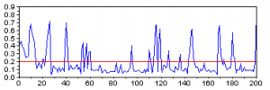
A look on the picture above will tell you that a threshold of about 0.2 might be good for discriminating the masts from the background. Once we apply it, there are at least two easy ways to derive the number of masts.
- Firstly, we could count the number of pixels over the threshold and divide it by four, which seems like roughly the average width of a mast.
answer = sum(img_line > 0.2)/4
The result is ~135.
- Secondly, we could count the number of times the pixel value crosses the 0.2 boundary:
answer = sum(img_line(2:$) > 0.2 & img_line(1:($-1)) <= 0.2);
Here the result will be 158.
2. Spectral approach
The discrete Fourier transform of a vector is a natural way for counting repeating peaks in the signal.
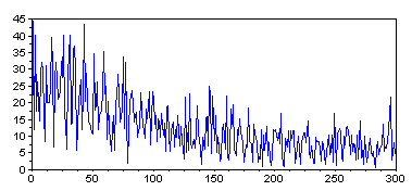
  ff = abs(fft(center(img_line)));
  plot(0:300, ff(1:301));
The interpretation of the resulting figure should, in theory, be simple. If the photo only contained n uniformly distributed masts, the spectrum would have one clear peak at n. In our case, unfortunately, things do not seem to be as easy. With some wishful thinking one might see major peaks around 50, 150 and 300. Now taking the previous results into consideration let us presume that 150 is the correct peak. Then 50 could correspond to the 50 "larger" masts on the image, and 300, perhaps, to the ropes.
3. Statistical approach
The original image is 1600 pixels wide. If the photo contained n masts, distributed uniformly along its width, a randomly chosen 32-pixel region would contain about n/50 masts on average. Therefore, let us select some of these random regions and count the number of masts in them manually. After multiplying the resulting numbers by 50 we should obtain estimates of the total number of masts.
  xbasc();
  rand("seed", 1);
  for i=1:9
    m = floor(rand()*(1600-32))+1;
    subplot(3,3,i);
    imshow(img([474:566], [m:(m+32)],:))
  end
Here are the estimates I got here: 200, 50, 50, 150, 150, 100, 100, 100, 100. The average comes at 111 with a standard deviation of about 50.
Summary
There are serious discrepances among the results produced by various approaches. However, if you attempt to count the masts manually, you will quickly discover that there is indeed an inherent degree of uncertainty in the number of visible masts, with the true number lying somewhere between 100 and 150. Consequently, the considered approaches to mast counting were not too far off, after all.
Tags: Fun, Image processing, Scilab, Travel
- Firstly, we could count the number of pixels over the threshold and divide it by four, which seems like roughly the average width of a mast.
-
The first step in the analysis of multivariate data is visualization. Histograms of attribute distributions, scatterplots, box-and-whiskers diagrams, parallel coordinate plots, self organizing maps, and even plots of happy faces - are all means of helping a human to visually comprehend multidimensional data and expoit the enormous power of the human brain to detect patterns. Of all these techniques, two-dimensional scatterplots are perhaps the most popular, as they tend to provide an especially "realistic" feel for the data. But when your data has more than two attributes (perhaps hundreds or thousands), how do you choose the two projection coordinates that would provide you with the "best angle" on the data?
The easiest answer to that question is, of course, to pick a pair of attributes Ai and Aj, and simply plot one versus the other. Unfortunately, this doesn't usually work well, especially when the dataset does have hundreds of attributes. Therefore, the most popular approach in practice is to use PCA and project the data onto the two largest principal components, which mostly results in a rather insightful image.
The PCA projection is, however, completely unsupervised. If your data has class labels assigned to points, PCA does not take them into account. No matter what is the labeling, PCA will always produce the same projection onto the coordinates with the highest variation. This might leave an improper impression that the two classes overlap a lot when in fact they do not. Therefore, this is not what you need. Usually, in the case of labeled data you expect from a scatterplot to provide an indication of how separated the two classes are from each other, and how difficult could it be to discriminate between them. It turns out that it is very easy to construct a linear projection with such properties.
The Linear classifier-based Scatterplot
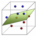
Assume there are two classes in the data and we are interested in a linear projection, that demonstrates how separated the classes are. Let us train a linear classifier to discriminate the two classes. It does not matter which algorithm you use, as long as it results in a separating hyperplane. Now naturally, the normal to this hyperplane is the main coordinate of interest to you: it is the direction along which the data will be classified linearly by your algorithm. If there is a coordinate for demonstrating separation, this must be it. The choice of the second projection coordinate does not matter much, so I would propose picking any direction orthogonal to the first.
When you have three classes you could select the first projection coordinate as the normal of a hyperplane, separating the first class from the second, and the second coordinate as the normal of a hyperplane, separating the first class from the third.
Finally, note that in general you need not limit yourself to linear classifiers only. Any classifier of the form
 will provide you with an informative coordinate projection function
  . This is a natural "supervised" alternative to kernel-PCA or SOM.
Naive supervised linear scatterplot (NS-plot)
To be somewhat more specific, here's a suggestion of a very simple implementation for the abovementioned idea. To avoid the use of a potentially complicated linear classifier training algorithm, let us just pick the vector connecting the means of the two classes as the first projection coordinate. The second coordinate is chosen at random and then orthogonalized with the first one. The Scilab code of the whole algorithm is therefore the following:
  // Input:
  //   X - the data matrix (instances in rows, attributes in columns)
  //   C - class assignments (C(i) is the class of instance X(i,:))
  mean_1 = mean(X(C ==  1, :), 'r')';
  mean_2 = mean(X(C == -1, :), 'r')';
  v1 = (mean_2 - mean_1)/norm(mean_2 - mean_1);
  v2 = rand(v1);
  v2 = v2 - v2'*v1*v1;
  v2 = v2/norm(v2);
  X_proj = X*[v1 v2];
  // Output:
  //   X_proj - the projected coordinates
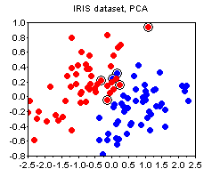
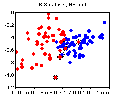
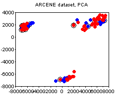
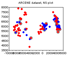
Notice how much simpler and more efficient it is than PCA. Despite the simplicity, I haven't seen the use of such a plot anywhere else, so let me coin the boring name NS-plot for it. Personal experience shows that the resulting plot is visually never much worse than a PCA plot, and most often the two plots complement each other. Let me illustrate that on two simple examples.
The IRIS dataset. The plots below show the PCA and the NS plots of the famous iris dataset (where I removed the first class). There is clearly no strong advantage of one plot over the other except that PCA is more difficult to compute.
The ARCENE dataset. The following plots depict the 1000-attribute ARCENE sample dataset. We can see how PCA prefers to stress the unsupervised clustering present in the dataset, thus potentially deemphasizing the specifics of class labeling. In this case, I would say, the PCA and the NS plots complement each other.
Bonus
Noticed the circled points on the plots above? This is one other small trick that I find quite useful, and that does not seem to be widely known. The circled points denote the "boundary" - these are the points whose nearest neighbor is of a different class than their own. The more boundary points there are - the more difficult is the classification problem. The boundary is not an absolute notion, because there are various ways to define distance between points. My suggestion would be to standardize all attributes and use the euclidean norm, unless you have good reasons to do something else (e.g. you a-priori know good weights for the attributes, etc).
Tags: Data analysis, Visualization
-
Everyone, who flies reasonably often has a chance to observe a remarkable effect: no matter how steep the roll angle of an airliner is during a turn, the tea in your cup will always stay parallel to the floor, and not to the ground. In the course of one recent unexpectedly long discussion on this topic, it turned out there is no much easily googleable material out there to refer to. I thought I'd create some, hence a somewhat longer post on an otherwise simple matter of minor relevance to my main affairs.
So, firstly, why doesn't tea orient itself parallel to the ground? To understand that, consider a pair of insightful examples. They should rid you of the incorrect intuitive assumption that it is gravity, which plays a defining role in the orientation of your tea.
Example 1: Water in the bucket
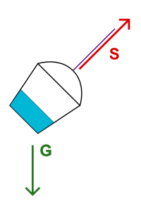
Consider the experiment described in the previous post about a water bucket on a string. No matter what you do with the bucket, as long as the string is at strain, the water will stay parallel to bottom of the bucket, and not to the ground. The explanation for that is the following. Water is affected by gravity G. The bucket is affected by gravity G and the strain of the string S. Therefore, from the frame of reference of the bucket, water experiences force G-(G+S) = -S, which pulls it towards the bottom of the bucket.
Example 2: Paragliders
You have probably seen paragliders in the air. If not, just search for "extreme paragliding" on youtube. Note that whatever the angle of the wing, the person is always hanging perpendicularly to it. Now if you'd hand him a bottle with water, the water would, naturally, also orient itself in parallel to the wing. The reason of that behaviour is the same as in the water bucket experiment, with the lift of the wing playing the same role as the strain of the string.
The main idea of both examples is that as long as the container and the object inside it are equally affected by gravity, it is not gravity that orients the object with respect to the container. More precisely, for the water to incline to the side, there must be some force acting on the container from that side.
The Airplane: A Simple Model
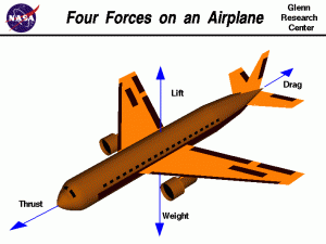
Let us now consider an idealized airplane. According to a popular model, an airplane in flight is affected by four forces: the thrust of the engines T, the drag due to air resistance D, the lift of the wings L and the gravitational weight of the airplane G. The glass of tea inside the airplane is, of course, only affected by gravity G. By applying the same logic as before, we can easily compute, that in the frame of reference of the airplane, the tea is experiencing acceleration F = G-(T+D+L+G) = -(T+D+L).However, once the airplane has attained constant speed (which is true for most of the duration of the flight), its thrust is completely cancelled by the air resistance, i.e. T+D = 0, in which case F = -L. It now remains to note that the lift force of the wings is always approximately perpendicular to the wings and thus to the floor of the airliner. The tea in your cup must therefore indeed be parallel to the floor.
The Airplane: A More Realistic Model
The model considered in the previous section is somewhat too simplistic. According to it there are no forces acting on the sides of the airplane whatsoever, and it should therefore be absolutely impossible to incline the tea in the cup to the side, which is, of course, not true for a real airplane. So, assuming a pilot would want to incline the tea and spill it, what would be his options?- Thrust. As noted above, tea must only be parallel to the floor when thrust is perfectly cancelled by drag and the plane is moving with constant speed. A rapid increase or decrease in thrust could therefore incline the tea towards or against the direction of flight. But of course, there is usually no need for such a maneuver during a passenger flight except for takeoff and landing.
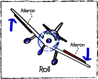
- Rotation. The model above does not consider the fact, that the pilot may use the ailerons and rudder to turn the airplane, rotating it around its axes. And of course, when the resulting rotation is abrupt enough, the tea could incline somewhat. However, during passenger flights the turns are always performed very smoothly, with rotation speeds around 1 degree per second. In fact it is risky, if not impossible to perform any hasty rotationary maneuvers on an airliner travelling at about 800km/h.
-
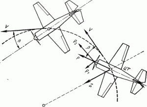
Slip. The simple model above considered the case when the air is flowing directly along the main axis of the airplane, which need not necessarily always be the case. The condition may be violated either due to a strong sidewind, or during a peculiar kind of a turn, where the airplane "slips" or "skids" on the side. In both cases, the airflow is exerting pressure on the side of the airplane's hull, which generates the so-called body lift. It is usually incomparably smaller than the lift of the wings, but nonetheless, it can incline the water to the side.
It is interesting to understand why you should almost never experience slip in an airliner. There are two reasons for that. Firstly, most airplanes have a degree of weathercock stability. Like a weathercock, an airplane with a vertical tail stabilizer tends to automatically orient itself into the direction of airflow and thus avoid slip. This effect is especially strong at the speed of a commercial airliner.
Secondly, if the weathercock effect is not enough to prevent slip, the pilot himself will always ensure that the slip is never too large by watching the slip-indicator (aka inclinometer) and coordinating the turn.
Why that? Because the airplane is not constructed, aerodynamically, to fly sideways. When the plane is moving sideways, the body of the plane blocks airflow over the trailing wing. So the wing loses lift and begins to drop. This naturally will put the airplane into a bank in the direction of the turn, but it does so at great cost in drag. When the slip is too large the lifting properties of the wings change so drastically that this might put the airplane at the risk of a crash.
Summary
Q: Why is the tea in an airliner parallel to the floor even when the airplane is turning?
A: It follows from the following three conditions, that must all be satisfied for a safe flight:- The forces of thrust and drag cancel each other and the airplane moves at a constant speed.
- The turns are performed smoothly.
- There is no slip: the air flows directly along the main axis of the airplane.
-
Most of us probably remember this experiment from high school physics lessons: you take a bucket on a string filled with water, spin it around your head and the water does not spill. "But how?" - you would ask in amazement. And the teacher would explain then:
"You see, the bucket is spinning, and this creates the so-called centrifugal force acting on the water, which cancels out gravity and thus keeps the water in the bucket". And you will have a hard time finding any other explanation. At least I failed no matter how hard I googled it.Unfortunately, this explanation looses an essential point of the experiment and I have seen people irreparaply braindamaged by the blind belief that it is only due to rotation and the resulting virtual centrifugal force that the water does not spill.
However, it is not quite the case. Let us imagine that the bucket has accidentally stopped right over your head and as a result, all centrifugal force has been immediately lost. Would the water spill? It will certainly fall down on your head, but it will do so together with the bucket. Thus, technically, the water will stay inside the bucket.
In fact, the proper way to enjoy the true magic of the experiment is not to swing the bucket in full circles, but rather let it swing back and forth as a pendulum (if you have a string and a beverage bottle nearby, you can do an experiment right now). One will then observe that even at the highest points of the swing, where the bottom of the bucket is at its steepest angle and the centrifugal force is nonexistant, the water stays strictly parallel to the bottom of the bucket, as if no gravity would act upon it. Why doesn't it spill? Clearly, the argument of centrifugal force cancelling gravity is inappropriate.
The proper explanation is actually quite simple and much more generic. We have two objects here: the bucket and the water in it. There is one (real) force acting on the water: gravity G. There are two (real) forces acting on the bucket: gravity G and the strain S of the string pulling the bucket perpendicularly to its bottom. (Note that the centrifugal force is not "real" and I do not consider it here, but if you wish, you may. Just remember then that it acts both on the water and the bucket.)
Now the question of interest is, how does water behave with respect to the bucket? That is, what force "pulls" the water towards the bucket and vice-versa. This can be easily computed by subtracting all forces acting on the bucket from all forces acting on the water. And the result is, of course, G - (S+G) = -S, i.e. a force, pulling the water directly towards the bottom of the bucket.A magical consequence of this argument is that gravity does not matter inside the bucket, as long as it can act on the bucket freely in the same way as on anything inside it. Nothing special about rotation here, really. It takes a while to realize.
Tags: Conspiracy, Experiment, Fun, Physics
-
Imagine that you have just derived a novel IQ test. You have established that for a given person the test produces a normally-distributed unbiased estimate of her IQ with variance 102. That is, if, for example, a person has true IQ=120, the test will result in a value from a N(120,102) distribution. Also, from your previous experiments you know that among all the people, IQ has a N(110,152) distribution.
One a sunny Monday morning you went out on a street and requested the first bypasser (whose name turned out to be John) to take your test. The resulting score was t=125. The question is: what can you conclude now about the true IQ of that person (assuming, of course, that there is such a thing as a "true IQ"). There are at least two reasonable approaches to this problem.
-
You could apply the method of maximum likelihood. Here's John, standing beside you, and you know his true IQ must be some real number a. The test produced an unbiased estimate of a equal to 125. The likelihood of the data (i.e. the probability of obtaining a test score of 125 for a given a) is therefore:
![Rendered by QuickLaTeX.com \[P[T=125|A=a]=\frac{1}{\sqrt{2\pi 10^2}}\exp\left(-\frac{1}{2}\frac{(125-a)^2}{10^2}\right)\]](https://fouryears.eu/wp-content/ql-cache/quicklatex.com-71cbad335e7c1df695c1e3fddcb59519_l3.png)
The maximum likelihood method suggests picking the value of a that maximizes the above expression. Finding the maximum is rather easy here and it turns out to be at a=125, which is pretty natural. You thus conclude that the best what you can say about John's true IQ is that it is approximately 125.
-
An alternative way of thinking is to use the method of maximum a-posteriori probability, where instead of maximizing likelihood
![Rendered by QuickLaTeX.com P[T=125|A=a]](https://fouryears.eu/wp-content/ql-cache/quicklatex.com-d636bf3ce38ceb5b2ca24cb3e5722fd0_l3.png) , you maximize the a-posteriori probability
, you maximize the a-posteriori probability ![Rendered by QuickLaTeX.com P[A=a|T=125]](https://fouryears.eu/wp-content/ql-cache/quicklatex.com-0fb0b91482de103b2722200ed4c1ffbb_l3.png) . The corresponding expression is:
. The corresponding expression is:
![Rendered by QuickLaTeX.com \begin{multiline} P[A=a|T=125] \sim P[T=125|A=a]\cdot P[A=a] = \\ = \frac{1}{\sqrt{2\pi 10^2}}\exp\left(-\frac{1}{2}\frac{(125-a)^2}{10^2}\right)\cdot \frac{1}{\sqrt{2\pi 15^2}}\exp\left(-\frac{1}{2}\frac{(110-a)^2}{15^2}\right) \end{multiline}](https://fouryears.eu/wp-content/ql-cache/quicklatex.com-783dc171af3ba91deedff337cb18da0b_l3.png)
Finding the required maximum is easy again, and the solution turns out to be a=120.38. Therefore, by this logic, John's IQ should be considered to be somewhat lower than what the test indicates.
Which of the two approaches is better? It might seem utterly unbelievable, but the estimate provided by the second method is, in fact, closer to the truth. The straightforward "125", proposed to by the first method is biased, in the sense that on average this estimate is slightly exaggerated. Think how especially unintuitive this result is from the point of view of John himself. Clearly, his own "true IQ" is something fixed. Why on Earth should he consider "other people" and take into account the overall IQ distribution just to interpret his own result obtained from an unbiased test?
To finally confuse things, let us say that John got unhappy with the result and returned to you to perform a second test. Although it is probably impossible to perform any real IQ test twice and get independent results, let us imagine that your test can indeed be repeated. The second test, again, resulted in a score of 125. What IQ estimate would you suggest now? On one hand, John himself came to you and this time you could regard his IQ as a "real" constant, right? But on the other hand, John is just a person randomly picked from the street, who happened to take your test twice. Go figure.
PS: Some additional remarks are appropriate here:
- Although I'm not a fan of The Great Frequentist-Bayesian War, I cannot but note that the answer is probably easier if John is a Bayesian at heart, because in this case it is natural for him to regard "unknown constants" as probability distributions and consider prior information in making inferences.
- If it is hard for you to accept the logic in the presented situation (as it is for me), some reflection on the similar, but less complicated false positive paradox might help to relieve your mind.
- In general, the correct way to obtain the true unbiased estimate is to compute the mean over the posterior distribution:
![Rendered by QuickLaTeX.com \[E[a|T=125] = \int a \mathrm{dP}[a|T=125]\]](https://fouryears.eu/wp-content/ql-cache/quicklatex.com-9ad6d3c21e08ac9a34351b754d264321_l3.png)
In our case, however, the posterior is symmetric and therefore the mean coincides with the maximum. Computing the mean by direct integration would be much more complicated.
Tags: Bayes, Paradox, Probability theory, Puzzle, Statistics
-
You could apply the method of maximum likelihood. Here's John, standing beside you, and you know his true IQ must be some real number a. The test produced an unbiased estimate of a equal to 125. The likelihood of the data (i.e. the probability of obtaining a test score of 125 for a given a) is therefore:
-
Two hardened criminals are taken to interrogation in separate cells.
They are offered the usual deal:
If neither confesses, both get one year probation.
If both confess, both do 5 years in jail.
If one confesses, he goes free but the other does 10 years hard time.Here's what actually goes through their minds:
"Okay, if neither of us confesses, we have to go back to the real world. But its so hard there!
But if I confess, he will kill me when he gets out.. so thats bad...
If both of us confess, then we can just get back to jail and continue our lives!"Note that it shares some similarities with the original...
Tags: Fun, Game theory
-
I bet most of you haven't heard of MDX, because it seems to be a technology that is difficult to stumble upon. It is not covered in university courses, not mentioned in the headlines of PC-magazine articles, and the corresponding google search returns about 20000 results, which makes it thousands (and even tens of millions) times less popular than most other related keywords. This is completely unfair. I believe MDX is compulsory knowledge for everyone who is educated in databases and data analysis enough to appreciate the virtues of both SQL queries and Excel-like spreadsheet processing. A famous quote by Alan Perlis says: "A language that doesn't affect the way you think about programming, is not worth knowing". In these terms, MDX is a language well worth knowing.
MDX stands for Multidimensional Expressions. It is a language for specifying computations and performing queries on a multidimensional database, which effectively provides the computing power of spreadsheets in the form of a query language. Although it is not possible to explain all of MDX in a blog post, I'll try to show the gist of it in a couple of examples. I hope it will raise at least some interest in those, who are patient enough to read to the end. To understand MDX you need some experience with spreadsheets, so I'll assume you do and use the analogies with Excel.
Multidimensional data. You use spreadsheets to work with tabular data, i.e. something like that:
Tartu Tallinn Jan 21 -1.0 °C -2.1 °C Jan 22 -0.2 °C -0.2 °C Jan 23 0.3 °C -0.2 °C Average temperatureThis is a two-dimensional grid of numbers. Each point in the grid can be indexed by a tuple (Date, City). A multidimensional database is essentially the same grid but without the limitation of two dimensions. For instance, if there are several methods of measuring temperature, you can add a new dimension and index each cell by a tuple (Date, City, MeasurementMethod). And if you wish to keep both the average temperature and humidity, you just add a fourth dimension MeasureType to the database and store both, etc. Once your database becomes multidimensional it becomes impossible to display all of it as a two-dimensional table, so you will have to explore it by slices. For example, if the database did indeed contain 4 dimensions (Date, City, MeasurementMethod, MeasureType) then the above table would be a slice of it for (MeasureType = Temperature, MeasurementMethod = Usual). The MDX query corresponding to the slice would look as follows:
  select
    { City.Tartu, City.Tallinn } on columns,
    { Date.Jan.21, Date.Jan.22, Date.Jan.23 } on rows
  where (MeasureType.Temperature, MeasurementMethod.Usual)
Cell calculations. The second thing you use spreadsheets for is to compute new cell values from the existing ones. For example, you might wish to augment the table above with a column showing the temperature difference between Tartu and Tallinn and a row showing the average temperature over three days:
Tartu Tallinn Difference Jan 21 -1.0 °C -2.1 °C 1.1 °C Jan 22 -0.2 °C -0.2 °C 0.0 °C Jan 23 0.3 °C -0.2 °C 0.5 °C Average -0.3 °C -0.83 °C 0.53 °C Average temperatureTo do that in Excel you would have to enter a formula for each cell in the new column and row. In MDX you analogously write:
  create member City.Difference as (City.Tartu - City.Tallinn)
  create member Date.Jan.Average as
         (Avg({ Date.Jan.21, Date.Jan.22, Date.Jan.23 }))
Note that once you have defined the new members, they apply to any slice of your data. I.e., you have just defined the way to compute City.Difference and Date.Jan.Average for all existing measure types and measurement methods. Moreover, many of the useful aggregate computations are already predefined for you. For example, the MDX server would implicitly understand that Date.Jan denotes be the aggregation (e.g. average) of values over all the days of January, and Date is the aggregation of values over all the dates ever. Similarly, City denotes the aggregation over all cities. Thus, selecting the average temperature over all cities in January is a matter of requesting
  select
  where (Date.Jan, City, MeasureType.Temperature,
         MeasurementMethod.Usual)
Filters, orders and more. You often need to query the data for things like "cities with the highest average temperature in January", or request to "order days by the temperature difference between Tartu and Tallinn". This is where both the power and complexity of MDX becomes visible. The first query would look as follows:
  select
    Filter(City.Members, Date.Jan == Max(Date.Jan)) on columns
  where (MeasureType.Temperature, MeasurementMethod.Usual)
Notice how much more expressive this is in comparison to the equivalent query you would have to come up with in SQL. Besides slicing, filtering and ordering, an MDX server can support lots of various generic data processing and analysis functions (here, the exact capabilities depend on the vendor). Thus, when properly tuned, even the tasks such as "selecting differentially expressed genes that play a significant role in a linear model for predicting cancer stage from microarray expression data" could become a matter of a single concise query.
Pretty cool, don't you think?
-
Consider the following excerpt from a recent article in the British Medical Journal:
Mike has only two children, and they are called Pat and Alex, which could equally be boys’ or girls’ names. In fact, Pat is a girl. What is the probability that Alex is a boy?
a 50%
b Slightly less than 50%
c Slightly more than 50%
d Between 60% and 70%
e Between 40% and 30%d—Although this could be about the relative popularity of ambiguous names for boys and girls or about subtle imbalances in the sex ratio, it is not meant to be. The clue to the correct answer is in thinking about what we do not know about the family and what we do know already, and applying this to the expected probabilities of girls and boys.
We do not know if Pat was born first or second. We do know that there are only two children and that Pat is a girl. I am assuming that in the population, 50% of children are girls.
The birth order and relative frequency of two child families are: boy, boy (25%), girl, girl (25%), boy, girl (25%) girl, boy (25%). We know Mike’s family does not have two boys, since Pat is a girl, so we are only left with three choices for families with at least one girl. Two of these pairs have a boy and one does not. Hence the probability that Alex is a boy is two thirds or 66.7%.
If we had been told that Pat was born first then the probability that Alex is a boy drops to 50%.
The well-known "Boy or Girl" paradox that is referenced in the fragment above is probably as old as the probability theory itself. And it is therefore quite amusing to see an incorrect explanation for it presented in a serious journal article. You are welcome to figure out the mistake yourself.
For completeness sake, here is my favourite way of presenting this puzzle:
In the following, let Mike be a randomly chosen father of two kids.
- Mike has two kids, one of them is a boy. What is the probability that the other one is a girl?
- Mike has two kids, the elder one is a boy. What is the probability that the other one is a girl?
- Mike has two kids. One of them is a boy named John. What is the probability that the other one is a girl?
- I came to visit Mike. One of his two kids, a boy, opened the door to me. What is the probability that Mike's other child is a girl?
- I have a brother. What is the probability that I am a girl?
- I have a brother named John. What is the probability that I am a girl?
You can assume that boys and girls are equiprobable, the births of two kids are independent events, a randomly chosen boy will be named John with probability p, and that a family may have two kids with the same name.
If you haven't tried solving these yet, give it a try. I'm pretty sure you won't do all 6 questions correctly on the first shot.
Tags: Fun, Paradox, Probability theory, Puzzle
Calendar
| M | T | W | T | F | S | S |
|---|---|---|---|---|---|---|
| « Jan | ||||||
| 1 | ||||||
| 2 | 3 | 4 | 5 | 6 | 7 | 8 |
| 9 | 10 | 11 | 12 | 13 | 14 | 15 |
| 16 | 17 | 18 | 19 | 20 | 21 | 22 |
| 23 | 24 | 25 | 26 | 27 | 28 | 29 |
| 30 | 31 | |||||
Recent Comments
Archives
- January 2024 (1)
- October 2019 (1)
- February 2019 (1)
- November 2018 (1)
- June 2018 (1)
- April 2018 (1)
- March 2018 (1)
- December 2017 (1)
- July 2017 (2)
- May 2017 (1)
- March 2017 (4)
- November 2016 (3)
- July 2016 (2)
- May 2016 (1)
- January 2016 (2)
- September 2015 (2)
- July 2015 (1)
- June 2015 (1)
- May 2015 (1)
- April 2015 (3)
- March 2015 (3)
- January 2015 (2)
- March 2014 (2)
- January 2014 (1)
- April 2013 (1)
- February 2013 (2)
- January 2013 (1)
- November 2012 (1)
- October 2012 (2)
- September 2012 (2)
- June 2012 (1)
- May 2012 (1)
- January 2012 (3)
- December 2011 (2)
- October 2011 (3)
- May 2011 (1)
- March 2011 (1)
- June 2010 (1)
- February 2010 (2)
- November 2009 (1)
- October 2009 (3)
- August 2009 (2)
- June 2009 (1)
- March 2009 (3)
- February 2009 (3)
- January 2009 (5)
- December 2008 (4)
- November 2008 (3)
- October 2008 (7)
- September 2008 (8)
