• Posted by Konstantin 07.06.2012 33 Comments

    The following text will only make sense to you if you know the technical details of Support Vector Machine learning.

    Having recently had to give some lectures (1,2,3,4) and exercise sessions (1,2,3,4) on linear classification in a machine learning course, I discovered that one of the most famous linear classification methods, the classical Support Vector Machine, does not seem to be fully specified in any of the prominent reference materials. Namely, the SVM learning procedure produces two parameters: the coefficient vector \bf\alpha and the bias term b. While the problem of finding \bf\alpha is typically explained in sufficient detail, the procedure of computing b is usually swept under the carpet.

    Here is, for example, what we see in the Vapnik's seminal work, the birthplace of SVMs (Section 10.2, page 411):

    Vapnik (page 411)According to my calculations this is plain incorrect, because the corresponding Kuhn-Tucker conditions (in the "soft margin" SVM that we are considering here) are actually:

        \[\alpha_t^0\left(\frac{1}{\gamma}\sum_{i=1}^\ell \alpha_i^0y_i(x_t * x_i) + b-1+\xi_i\right) = 0\]

    The important difference is the presence of the \xi_i term, which is unknown, hence the equation is not useful for finding b. Later on, the reader is also presented with the following summarizing description of the algorithm:

    Vapnik (page 425)Do you see any mention of the way to compute b? I would expect the author to be somewhat more helpful with respect to this detail, which is obviously important for anyone willing to implement their own version of SVM.

    OK, that was an old book, let's take a look at some newer materials. The two books which could be regarded as authoritative sources on the subject of SVMs are probably "An Introduction to Support Vector Machines" and "Kernel Methods for Pattern Analysis". Here is what the first book tells us about computing b (Proposition 6.11, page 106):

    Cristianini (page 106)

    This suggests that in order to compute b we need to find \alpha_i^*, such that C>\alpha_i^*>0, i.e. there must exist at least one training point lying exactly on the margin. Although in most practical situations such support vectors will indeed exist, it is also theoretically possible that there won't be any, i.e. not a single support vector will lie exactly on the margin. Thus, for purposes of implementing SVMs, the provided specification is incomplete.

    The same problem is present in the second book:

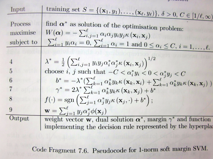
    Shawe-Taylor

    Take a careful look at lines 5-6, which claim that in order to compute b we need to choose i,j such that the corresponding \alpha_i, \alpha_j are strictly between 0 and C. This is not necessarily true for any \alpha_i.

    So then, what is the proper, fully general way of computing b? Of course, it is not too hard to derive, and thus makes for a great course homework exercise (e.g. Exercise 4 here). If you managed to read up to this point, I presume you should be motivated enough to try solving it. If you give up, you are welcome to consult my sample solution (Exercise 4, page 7).

    Tags: , , ,

  • Posted by Konstantin 04.12.2011 1 Comment

    There is one rule of thumb that I find quite useful and happen to use fairly often. It is probably not widely known nor described in textbooks (I stumbled upon it on my own), so I regularly have to explain it.  Next time I'll just point out to this post.

    The rule is the following: a proportion estimate obtained on a sample of n points should only be trusted up to an error of \frac{1}{\sqrt{n}}.

    For example, suppose that you read in the newspaper that "25% of students like statistics". Now, if this result has been obtained from a survey of 64 participants, you should actually interpret the answer as 0.25\pm\frac{1}{\sqrt{64}}, that is, 0.25\pm 0.125, which means that the actual percentage lies somewhere between 12.5% and 37.5%.

    As another example, in machine learning, you often get to see cases where someone evaluates two classification algorithms on a test set of, say, 400 instances, measures that the first algorithm has an accuracy of 90%, the second an accuracy of, say, 92%, and boldly claims the dominance of the second algorithm. At this point, without going deeply into statistics, it is easy to figure that 1/\sqrt{400} should be somewhere around 5%, hence the difference between 90% and 92% is not too significant to celebrate.

    The Explanation

    The derivation of the rule is fairly straightforward. Consider a Bernoulli-distributed random variable with parameter p. We then take an i.i.d. sample of size n, and use it to estimate \hat p:

        \[\hat p = \frac{1}{n}\sum_i X_i\]

    The 95% confidence interval for this estimate, computed using the normal approximation is then:

        \[\hat p \pm 1.96\sqrt{\frac{p(1-p)}{n}}\]

    What remains is to note that 1.96\approx 2 and that \sqrt{p(1-p)} \leq 0.5. By substituting those two approximations we immediately get that the interval is at most

        \[\hat p \pm \frac{1}{\sqrt{n}}\]

    Limitations

    It is important to understand the limitations of the rule. In the cases where the true proportion estimate is p=0.5 and n is large enough for the normal approximation to make sense (20 is already good), the one-over-square-root-of-n rule is very close to a true 95% confidence interval.

    When the true proportion estimate is closer to 0 or 1, however, \sqrt{p(1-p)} is not close to 0.5 anymore, and the rule of thumb results in a conservatively large interval.

    In particular, the true 95% confidence interval for p=0.9 will be nearly two times smaller (\approx 0.6/\sqrt{n}). For p=0.99 the actual interval is five times smaller (\approx 0.2/\sqrt{n}). However, given the simplicity of the rule, the fact that the true p is rarely so close to 1, and the idea that it never hurts to be slightly conservative in statistical estimates, I'd say the one-over-a-square-root-of-n rule is a practically useful tool in most situations.

    Use in Machine Learning

    The rule is quite useful to quickly interpret performance indicators of machine learning models, such as precision, accuracy or recall, however, you should make sure you understand what proportion is actually being computed for each metric. Suppose we are evaluating a machine learning model on a test set of 10000 elements, 400 of which were classified as "positive" by the model. We measure the accuracy of the model by computing a proportion of correct predictions on the whole set of 10000 elements. Thus, the n here is 10000 and we should expect the confidence intervals of the resulting value to be under 1 percent point. However, the precision of the model is measured by computing the proportion of correct predictions among the 400 positives. Here n is actually 400 and the confidence intervals will be around 0.05.

    The rule can also be used to choose the size of the test set for your model. Despite the popular tradition, using a fraction of your full dataset for testing (e.g. "75%/25% split") is arbitrary and misguided. Instead, it is the absolute size of the test sample that you should care most about. For example, if you are happy with your precision estimates to be within a 1% range, you only need to make sure your test set would include around 10000 positives. Wasting an extra million examples for this estimate will increase the quality of your estimate, but you might be better off leaving these examples for model training instead.

    Tags: , ,

  • Posted by Konstantin 12.10.2011 16 Comments

    The Receiver Operating Characteristic Area Under the Curve (ROC AUC) is a measure of classifier performance, which is widely used in machine learning. Unfortunately, the obscure way the concept is explained in most sources makes it fairly hard to grasp its intuitive meaning. The name "area under the curve" itself is ill-conceived and is utterly useless in helping the intution. The aim of this post is to aid those struggling with the concept, and also present a simple and intuitive interpretation of the ROC AUC metric as the "average positive rank" which I, so far, have not seen stated explicitly elsewhere.

    To facilitate explanation, let us consider a hypothetical classification problem: classifying chocolate bars to "very good" or "just OK" (hereby we presume a chocolate bar may not be considered "bad" by definition of chocolate). Suppose we have a sample of particular chocolate bar types, for which we have carefully assigned the proper classification, e.g.:

    Item Class
    Mars 0
    Milka 1
    Kalev 0
    Lindt 1
    Ferrero-Rocher 1
    Laima 0
    Hershey's 0

    where class label "1" denotes "very good" and "0" means "just OK". Suppose we have derived a classifier which, based on some features of a chocolate bar, such as its chocolate content, packaging, country of origin, etc, attempts to assign a "goodness score" which should resemble our notion of goodness. For concreteness' sake, let us say the classifier assigned the following scores:

    Item True class Assigned score
    Milka 1 8
    Mars 0 5
    Lindt 1 3
    Ferrero-Rocher 1 3
    Kalev 0 1
    Laima 0 -3
    Hershey's 0 -5

    How do we assess the goodness of such a classifier? The "ROC approach" suggests we do the following. First, we shall plot a ROC curve. To do that, we order the chocolate bars according to their assigned score (this is already done in the table above) and use this ordering to write out the vector of the class labels (the "sorted prediction vector"):

    Highest rated item's true class Lowest rated item's true class
    1 0 1 1 0 0 0

    Obviously, the best possible classifier would order the instances so that all the ones would be on the left of all the zeroes. The particular classifier we chose here looks good, but not perfect.

    Next, we use the obtained vector to plot the ROC curve. To do this plot, forget all of the "True Positive Rate" and "False Positive Rate" nonsense you might have read about in most textbooks, and follow the following simple recipe:

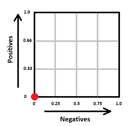
    1. Draw a square with sides of length 1. Denote its its lower left corner as the "origin", its horizontal axis as "the negatives" and its vertical axis as "the positives". Split the negatives axis in as many parts as there are examples of class "0" in the dataset. Split the positives axis in as many parts as there are examples of class "1" in your dataset. In our case, the square will look as follows:

      The ROC square

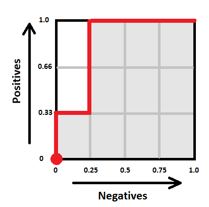
    2. Next, take the sorted prediction vector, and draw a path, starting from the origin. For each "1" in the sorted prediction vector, the path will move one step "up", and for each "0" in the vector, the path will move one step "right" (note that if you have multiple predictions with the same score, make all the corresponding "up" and "right" moves at once by drawing the corresponding diagonal). In our case, the path goes ("up", "right", "up", "up", "right", "right", "right") and hence looks as follows:

      ROC curve

    Voilà, this is your ROC curve. Obviously, the "perfect" classifier would make all the "up" steps first and the "right" steps last, hence the ideal ROC curve looks like a perfect corner. A random classifier would mix his "up" and "right" steps randomly, and the curve would most probably follow a diagonal-ish path. The one-number summary of the "goodness" of such a path is the "area under the curve" (coloured gray here), which will be 1.0 for the ideal case, and somewhere around 0.5 for the worst case. In our case the area is 10/12 ~ 0.83.

    Here comes the important question — what does this number actually mean? One good answer is given by the following probabilistic interpretation:

    The area under ROC curve specifies the probability that, when we draw one positive and one negative example at random, the decision function assigns a higher value to the positive than to the negative example.

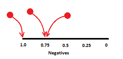
    There is, however, yet another, to my mind even more intuitive, interpretation. Define the rank of a positive example as the proportion of negative examples "to the right of it" in the sorted prediction vector. For example, if the sorted prediction vector is (1, 0, 0, 0, 0), then the rank of the sole positive item there is 1.0 (all negative examples are to the right). If the sorted prediction vector is (0, 0, 1, 0, 0), the rank is 0.5 (half of negative examples is to the right), and if the vector is (0, 0, 0, 0, 1), the rank is 0. In our chocolate bar example, the ranks of the positive examples are the following:

    Highest rated item's true class Lowest rated item's true class
    Sorted prediction vector 1 0 1 1 0 0 0
    Rank 1.0 0.75 0.75

    The "rank" thus denotes where would a classifier position a given positive item within the set of negative examples, whether closer to the "left" (rank 1) or closer to the "right" (rank 0).

    Now the average rank of all the positive examples seems like a reasonable metric of classifier performance, doesn't it? In fact, is exactly the ROC AUC! Now the value of 0.80 ROC score can be interpreted intuitively as follows: "the average positive example has about 20% of negative examples scored higher than it". This, so far, seems to me personally to be the "simplest" interpretation of the ROC AUC. So write it down:

    ROC AUC is the average positive rank.

    Tags: , ,

  • Posted by Konstantin 16.03.2011 No Comments

    This is a (slightly modified) write-up of a part of a lecture I did for the "Welcome to Computer Science" course last semester.

    Part I. Humans Discover the World

    How it all started

    Millions of years ago humans were basically monkeys. Our ape-like ancestors enjoyed a happy existence in the great wide world of Nature. Their life was simple, their minds were devoid of thought, and their actions were guided by simple cause-and-effect mechanisms. Although for a modern human it might seem somewhat counterintuitive or even hard to imagine, the ability to think or understand is, in fact, completely unnecessary to succesfully survive in this world. As long as a living creature knows how to properly react to the various external stimuli, it will do just fine. When an ape sees something scary — ape runs. When an ape seems something tasty — ape eats. When an ape sees another ape — ape acts according to whatever action pattern is wired into its neural circuits. Does the ape understand what is happening and make choices? Not really — it is all about rather basic cause and effect.

    As time went by, evolution blessed our ape-like ancestors with some extra brain tissue. Now they could develop more complicated reaction mechanisms and, in particular, they started to remember things. Note that, in my terminology here, "remembering" is not the same as "learning". Learning is about simple adaptation. For example, an animal can learn that a particular muscle movement is necessary to get up on a tree — a couple of failed attempts will rewire its neural circuit to perform this action as necessary. One does not even need a brain to learn — the concentration of proteins in a bacteria will adjust to fit the particular environment, essentially demonstrating a learning ability. "Remembering", however, requires some analytical processing.

    Remembering

    It is easy to learn to flex a particular finger muscle whenever you feel like climbing up a tree, but it is a totally different matter to actually note that you happen to regularly perform this action somewhy. It is even more complicated to see that the same finger action is performed both when you climb a tree and when you pick a banana. Recognizing such analogies between actions and events is not plain "learning" any more. It is not about fine-tuning the way a particular cause-and-effect reflex is working. It is a kind of information processing. As such, it requires a certain amount of "memory" to store information about previous actions and some pattern analysis capability to be able to detect similarities, analogies and patterns in the stored observations. Those are precisely the functions that were taken over by the "extra" brain tissue.

    So, the apes started "remembering", noticing analogies and making generalization. Once the concept of "grabbing" is recognized as a recurring pattern, the idea of grabbing a stone instead of a tree branch is not far away. Further development of the brain lead to better "remembering" capabilities, more and more patterns discovered in the surrounding world, which eventually lead to the birth of symbolic processing in our brains.

    Symbols

    What is "grabbing"? It is an abstract notion, a recurring pattern, recognized by one of our brain circuits. The fact that we have this particular circuit allows us to recognize further occurrences of "grabbing" and generalize this idea in numerous ways. Hence, "grabbing" is just a symbol, a neural entity that helps our brains to describe a particular regularity in our lives.

    As time went by, prehistoric humans became aware (or, let me say "became conscious") of more and more patterns, and developed more symbols. More symbols meant better awareness of the surrounding world and its capabilities (hence, the development of tools), more elaborate communication abilities (hence, the birth of language), and, recursively, better analytic abilities (because using symbols, you can search for patterns among patterns).

    Symbols are immensely useful. Symbols are our way of being aware of the world, our way of controlling this world, our way of living in this world. The best thing about them is that they are easily spread. It may have taken centuries of human analytical power to note how the Sun moves along the sky, and how a shadow can be used to track time. But once this pattern has been discovered, it can be recorded and used infinitely. We are then free to go searching for other new exciting patterns. They are right in front of us, we just need to look hard. This makes up an awesome game for the humankind to play — find patterns, get rewards by gaining more control of the world, achieve better life quality, feel good, everyone wins! Not surprisingly, humans have been actively playing this game since the beginning of time. This game is what defines humankind, this is what drives its modern existence.

    Science
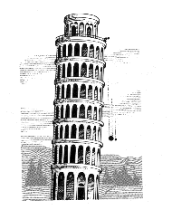
    Galelio's experiment

    "All things fall down" — here's an apparently obvious pattern, which is always here, ready to be verified. And yet it took humankind many years to discover even its most basic properties. It seems that the europeans, at least, did not care much about this essential phenomenon until the XVIIth century. Only after going through millenia self-deception, followed by centuries of extensive aggression, devastating epidemics, and wild travels, the europeans found the time to sit down and just look around. This is when Galileo found out that, oh gosh, stuff falls down. Moreover, it does so with the same velocity independently of its size. In order to illustrate this astonishing fact he had to climb on to the tower of Pisa, throw steel balls down and measure the fall time using his own heartbeat.

    In fact, the late Renaissance was most probably the time when europeans finally became aware of the game of science (after all, this is also a pattern that had to be discovered). People opened their eyes and started looking around. They understood that there are patterns waiting to be discovered. You couldn't see them well, and you had to look hard. Naturally, and somewhat ironically, the sky was the place they looked towards the most.

    Patterns in the Sky

    Tycho Brahe

    Tycho Brahe, a contemporary of Galileo, was a rich nobleman. As many other rich noblemen of his time, he was excited about the sky and spent his nights as an astronomer. He truly believed there are patterns in planetary motions, and even though he could not see them immediately, he carefully recorded daily positions of the stars and planets, resulting in a vast dataset of observations. The basic human "remembering" ability was not enough anymore — the data had to be stored on an external medium. Tycho carefully guarded his measurements, hoping to discover as much as possible himself, but he was not the one to find the pattern of planetary motion. His assistant, Johannes Kepler got a hold of the data after Tycho's death. He studied the data and came up with three simple laws which described the movements of planets around the Sun. The laws were somewhat weird (the planets are claimed to sweep equal areas along an ellipse for no apparent reason), but they fit the data well.
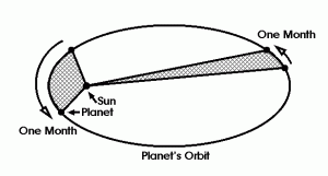
    Kepler's Laws

    This story perfectly mirrors basic human pattern discovery. There, a human first observes the world, then uses his brain to remember the observations, analyze them, find a simple regularity, and come up with an abstract summarizing symbol. Here the exact same procedure is performed on a larger scale: a human performs observations, a paper medium is used to store them, another human's mind is used to perform the analysis, the result is a set of summarizing laws.
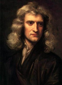
    Isaac Newton

    Still a hundred years later, Isaac Newton looked hard at both Galileo's and Kepler's models and managed to summarize them further into a single equation: the law of gravity. It is somewhat weird (everything is claimed to be attracted to everything for no apparent reason), but it fits the data well. And the game is not over yet, three centuries later we are still looking hard to understand Gravity.

    Where are we going

    As we play the game, we gradually run out of the "obvious" patterns. Detecting new laws of nature and society becomes more and more complicated. Tycho Brahe had to delegate his "memory" capabilities to paper. In the 20th century, the advent of automation helped us to delegate not only "memory", but the observation process itself. Astronomers do not have to sit at their telescopes and manually write down stellar positions anymore — automated radar arrays keep a constant watch on the sky. Same is true of most other science disciplines to various extents. The last part of this puzzle which is not fully automated yet is the analysis part. Not for long...

    Part II. Computers Discover the World

    Manufactured life

    Vacuum tube

    The development of electricity was the main industrial highlight of the XIXth century. One particularly important invention of that century was an incredibly versatile electrical device called the vacuum tube. A lightbulb is a vacuum tube. A neon lamp is a vacuum tube. A CRT television set is a vacuum tube. But, all the fancy glowing stuff aside, the most important function of a vacuum tube turned out to be its ability to act as an electric current switcher. Essentially, it allowed to hardwire a very simple program:

    if (wire1) then (output=wire2) else (output=wire3)

    It turns out that by wiring thousands of such simple switches together, it is possible to implement arbitrary algorithms. Those algorithms can take input signals, perform nontrivial transformations of those signals, and produce appropriate outputs. But the ability to process inputs and produce nontrivial reactions is, in fact, the key factor distinguishing the living beings from lifeless matter. Hence, religious, spiritual, philosophical and biological aspects aside, the invention of electronic computing was the first step towards manufacturing life.

    Of course, the first computers were not at all like our fellow living beings. They could not see or hear, nor walk or talk. They could only communicate via signals on electrical wires. They could not learn — there was no mechanisms to automaticaly rewire the switches in response to outside stimuli. Neither could they recognize and "remember" patterns in their inputs. In general, their hardwired algorithms seemed somewhat too simple and too predictable in comparison to living organisms.
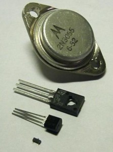
    Transistors

    But development went on with an astonishing pace. The 1940's gave us the most important invention of the XXth century: the transistor. A transistor provides the same switching logic as a vacuum tube, but is tiny and power-efficient. Computers with millions and billions of transistors became gradually available. Memory technologies caught up: bytes grew into kilobytes, megabytes, gigabytes and terabytes (expect to see a cheap petabyte drive at your local computer store in less than 5 years). The advent of networking and the Internet, multicore and multiprocessor technologies followed closely. Nowadays the potential for creating complex, "nontrivial" lifelike behaviour is not limited so much by the hardware capabilities. The only problem left to solve is wiring the right program.

    Reasoning

    The desire to manufacture "intelligence" surfaced early on in the history of computing. A device that can be programmed to compute, must be programmable to "think" too. This was the driving slogan for computer science research in most of the 1950-1980s. The main idea was that "thinking", a capability defining human intellectual superiority over fellow mammals, was mainly related to logical reasoning.

    "Socrates is a man. All men are mortal. => Hence, Socrates is mortal."

    As soon as we teach computers to perform such logical inferences, they will become capable of "thinking". Many years of research have been put in to this area and it was not in vain. By now, computers are indeed quite successful at performing logical inference, playing games and searching for solutions of complex discrete problems. But the catch is, this "thinking" does not feel like being proper "intelligence". It is still just a dumb preprogrammed cause-and-effect thing.

    The Turing Test
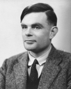
    Alan Turing

    A particular definition of "thinking" was provided by Alan Turing in his Turing test: let us define intelligence as a capability of imitating a human in a conversation, so that it would be indistinguishable from a real human. This is a hard goal to pursue. It obviously cannot be achieved by a bare logical inference engine. In order to imitate a human, computer has to know what a human knows, and that is a whole lot of knowledge. So, perhaps intelligence could be achieved by formalizing most of human knowledge within a powerful logical inference engine? This has been done, and done fairly well, but sadly, this still does not resemble real intelligence.

    Reasoning by Analogy
    Optical character recognition

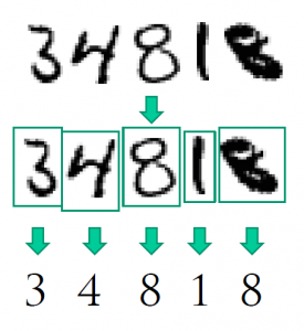
    While hundreds of computer science researchers were struggling hard to create the ultimate knowledge-based logical system, real-life problems were waiting to be solved. No matter how good the computer became at solving abstract logical puzzles, he seemed helpless when faced with some of the most basic human tasks. Take, for example, character recognition. A single glimpse at a line of handwritten characters is enough for a human to recognize the letters (unless it is my handwriting, of course). But what logical inference should the computer do to perform it? Obviously, humans do not perform this task using reasoning, but rely on intuition instead. How can we "program" intuition?

    The only practical way to automate character recognition turned out to be rather simple, if not to say dumb. Just store many examples of actual handwritten characters. Whenever you need to recognize a character, find the closest match in that database and voila! Of course, there are details which I sweep under the carpet, but the essence is here: recognition of characters can only be done by "training" on a dataset of actual handwritten characters. The key part of this "training" lies, in turn, in recognizing (or defining) the analogies among letters. Thus, the "large" task of recognizing characters is reduced to a somewhat "smaller" task of finding out which letters are similar, and what features make them similar. But this is pattern recognition, not unlike the rudimentary "remembering" ability of the early human ancestors.

    The Meaning of Life

    Please, observe and find the regularity in the following list:

    • An ape observes its actions, recognizes regularities, and learns to purposefully grab things.
    • Galileo observes falling bodies, recognizes regularities, and leans to predict the falling behaviour.
    • Tycho Brahe observes stars, Johannes Keper recognizes regularities, and learns to predict planetary motion.
    • Isaac Newton observes various models, recognizes regularities, and develops a general model of gravity.
    • Computer observes handwritten characters, recognizes regularities, and learns to recognize characters.
    • Computer observes your mailbox, recognizes regularities, and learns to filter spam.
    • Computer observes natural language, recognizes regularities, and learns to translate.
    • Computer observes biological data, recognizes regularities, and discovers novel biology.

    Unexpectedly for us, we have stumbled upon a phenomemon, which, when implemented correctly, really "feels" like true intelligence. Hence, intelligence is not about logical inference nor extensive knowledge. It is all about the skill of recognizing regularities and patterns. Humans have evolved from preprogrammed cause-and-effect reflexes through simple "remembering" all the way towards fairly sophisticated pattern analysis. Computers now are following a similar path and are gradually joining us in The Game. There is still a long way to go, but we have a clear direction: The Intelligence, achieving which means basically "winning" The Game. If anything at all, this is the purpose of our existence - discovering all the regularities in the surrounding world for the sake of total domination of Nature. And we shall use the best intelligence we can craft to achieve it (unless we all die prematurely, of course, which would be sad, but someday some other species would appear to take a shot at the game).

    Epilogue. Strong AI

    There is a curious concept in the philosophical realms of computer science — "The Strong AI Hypothesis". It relates to the distinction between manufacturing "true consciousness" (so-called "strong AI") and creating "only a simulation of consciousness" (the "weak AI"). Although it is impossible to distinguish the two experimentally, there seems to be an emotional urge to make the distinction. This usually manifests in argumentation of the following kind: "System X is not true artificial intelligence, because it is a preprogrammed algorithm; Humans will never create true AI, because, unlike us, a preprogrammed algorithm will hever have free will; etc."

    Despite the seemingly unscientific nature of the issue, there is a way to look at it rationally. It is probably true that we shall never admit "true intelligence" nor "consciousness" to anything which acts according to an algorithm which is, in some sense, predictable or understandable by us. On the other hand, every complex system that we ever create, has to be made according to clearly understandable blueprints. The proper way of phrasing the "Strong AI" question is therefore the following: is it possible to create a system, which is built according to "simple" blueprints, and yet the behaviour of which is beyond our comprehension.
    Cellular automaton

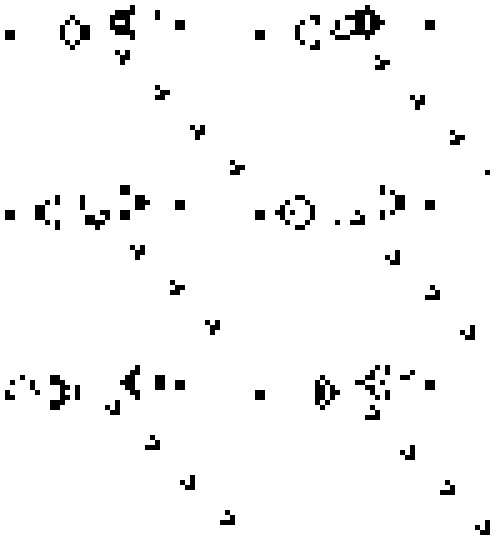
    The answer to this question is not immediately clear, but my personal opinion is that it is a strong "yes". There are at least three kinds of approaches known nowadays, which provide a means for us to create something "smarter" than us. Firstly, using everything fractal, cellular, and generally chaotic is a simple recipe for producing uncomprehensibly complex behaviour from trivial rules. The problem with this approach, however, is that there is no good methodology for crafting any useful functions into a chaotic system.


    The second candidate is anything neural — obviously the choice of Mother Nature. Neural networks have the same property of being able to demonstrate behaviour, which is not immediately obvious from the neurons or the connections among them. We know how to train some types of networks and we have living examples to be inspired by. Nonetheless, it is still hard to actually "program" neural networks. Hence, the third and the most promising approach — general machine learning and pattern recognition.

    The idea of a pattern recognition-based system is to use a simple algorithm, accompanied by a huge dataset. Note that the distinction between the "algorithm" and the "dataset" here draws a clear boundary between two parts of a single system. The "algorithm" is the part which we need to understand and include in our "blueprints". The "data" is the remaining part, which we do not care knowing about. In fact, the data can be so vast, that no human is capable of grasping it completely. Collecting petabytes is no big deal these days any more. This is a perfect recipe for making a system which will be capable of demonstrating behaviour that would be unpredictable and "intelligent" enough for us to call it "free will".

    Think of it...

    Tags: , , , ,

  • Posted by Swen 13.02.2010 2 Comments

    The recent blog post "Machine Learning in Mordor" is an excellent example of inherent bias in error estimation methods. Let us consider a standard classification task for simplicity. Then a good machine learning practice is first to find a classifier that is optimal or near-optimal on the training set. Recall that for a fixed classifier the training error is a Monte-Carlo estimate of the generalisation error - the average error that the classifier makes if the data is drawn independently from some unknown but fixed distribution. However, as soon as we choose to minimise the training error, the estimate becomes biased. The training error underestimates the generalisation error.

    To avoid this the data is usually split into two separate sets: training data and validation data. If we choose the classifier according to the training data and later estimate the generalisation error on the validation data, the bias disappears and we should be in good shape. Moreover for certain classification methods, such as Support Vector Machines, it is possible to prove that the training error and the generalisation error are closely connected. That is, we can prove formulae

    GeneralisationError <= TrainingError + F(n)

    where F(n) is a bias term that depends on size of the training sample. Although both of these arguments are formally correct, they are actually void in certain practical settings.

    For instance, student Bughrorc who split the data into a 15 element training and 5 element test set did not do anything wrong, but yet his classification algorithm is likely to perform inferior to the method proposed by Aghargh.

    One could argue that Bughrorc made a mistake and used the validation set for choosing between several competing classifiers and thus, for the same reasoning as explained above, the estimate on the generalisation error is now an underestimation. However, this is only a partial explanation.

    Imagine a standard no-free-lunch setting, where the labels to the data are assigned randomly so that 80% spells are good and 20% of the spells are bad. Moreover, assume that Bughrorc chooses only one classification algorithm on the training set and later uses the validation set for estimating the generalisation error. As the sample is small, the validation error might be zero again. Is the estimate free of bias now and is Bughrorc safe?

    Actually not. As weird as it seems, statistical estimates depend on your intention and potential behaviour. If Bughrorc sees a small error estimate and accepts it as a correct one, it does not mean that this is unbiased eventhough the validation was properly done. To verify whether the estimate is biased or not, Bughrorc has to explore his deeper thoughts. If he can solemnly promise that a larger validation error would not had discouraged him to drop the experiment, then the validation error is indeed unbiased (but wrong). However, if a larger validation error would have stopped him from using the classifier, the same result is biased (and wrong) - whenever Bughrorc accepts the validation error it is necessarily small and thus the validation error actually underestimates the generalisation error.

    As most of us are sane enough not to use a classifier with an estimated classification error near 100% or even near 50%, the validation error is biased for all practical purposes.

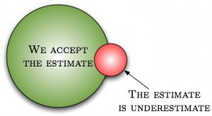
    Surprisingly enough this bias can be estimated. Let us first fix a conservative point estimate for the validation error that is smaller than the actual generalisation error on at most 5% cases, if the validation samples are independently from the actual distribution. For example, assume that we are willing to accept the 20% classification error and the classification problem is easy - for a randomly drawn sample, the validation error is below 20 with probability 95%. Now even though we shall tend to unfairly reject all cases where the validation error overestimates the generalisation error (thus biasing our estimate towards underestimation), the fraction of such cases is at most 5/95=5.3%. Consequently, the estimate is a safe overestimate with confidence 94.7%.

    Easy machine learning problem

    Easy machine learning problem

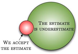
    On the other hand, if the classification problem is difficult, say, the validation error is below 20% with probability 4%, then the situation is completely different. Since the fraction of cases where the validation fails is larger than the fraction of cases we accept the estimate, all cases where we accept the estimate might be incorrect. Consequently, the estimate is a safe overestimate with confidence 0%.

    Difficult machine learning problem

    Difficult machine learning problem

    As a final remark, note that if the validation set is small and the classification task is difficult then validation error is below accepting threshold with significant probability. For the non-free lunch Mordor case, the acceptance probability is 80% for a single point and thus we underestimate the result in 80% possible cases. If the validation set is large, then such a small error is achieved with insignificant probability and the question whether we should or should not continue does not occur "at all". In other words, the smaller is our acceptable error rate, the larger must be the validation set to compensate the rejection bias.

    Tags: , ,

  • Posted by Konstantin 21.11.2009 No Comments

    In the recent weeks I had to give a few introductory lectures on supervised machine learning within Jaak's data mining course. I also provided the students some home assignments, and there it was especially tricky to find a simple, fun and discussable exercise, which might help to form some intuition regarding the inherent difficulties of learning from data such as overfitting, multiple testing, and the like. The following is what I came up with and I find it a rather successful creation. It is remarkable that of the 80 students participating in the course only 4 or so came up with the correct answer 🙂

    The Riddle

    After the lecture on supervised machine learning at the University of Mordor, the teacher, Sauron, gave the students a dataset of the following form:

                1) ABACDAFXYZ    -> good
                2) CEGXEAELWMN   -> good
                3) NUWAB         -> bad
                        ...
               20) QRELAZMNPCXA  -> good

    The inputs were seemingly arbitrary strings of latin characters: these were the terrible spells known only to Sauron and chosen by Sauron at random from his Great Book of Terrible Spells. The output was a binary variable, classifying each spell as good or bad. There were 20 observations in total in the dataset.

    The students were given a task: on the basis of this data, come up with a generic spell classifier. Sauron promised to test their result on the next lecture as follows: he will pick another random terrible spell from the book and require each student to make a prediction. The student whose prediction is wrong will have to jump down from the tower as a punishment.

    The first student, Aghargh, who happened to be slacking on the lecture, couldn't come up with any smart ways to solve the task, so he ended up just counting the proportion of "good" and "bad" spells in the dataset. Having observed that 16 of the 20 spells were "good", he decided to predict "good" when asked.

    The second student, Bughrorc, chose a smarter way. Firstly, he converted each string into a vector of binary attributes — one attribute for each letter, having value "1" if that letter was present in the corresponding spell and "0" otherwise. He then split the data randomly into a training set (15 instances) and a test set (5 instances), and attempted training various classifiers using the MordorMiner software. After some experimenting he finally found five classifiers that could predict all of the training examples correctly. One of these also predicted all of the testing examples correctly. He decided to use this classifier on the forthcoming test.

    On the day of testing, Sauron asked the students to classify the spell YOZAZA. Aghargh, as he decided, provided the answer "good". Bughrorc's classifier analyzed the string and claimed that the answer should be "bad"

    Which of the students, do you think, might have a better chance of not jumping from the tower? Why? Can you quantify your answer?

    Tags: , , ,

  • Posted by Konstantin 07.12.2008 7 Comments

    Logic versus Statistics

    Consider the two algorithms presented below.

    Algorithm 1:

       If, for a given brick B,
          B.width(cm) * B.height(cm) * B.length(cm) > 1000
       Then the brick is heavy

    Algorithm 2:

       If, for a given male person P,
          P.age(years) + P.weight(kg) * 4 - P.height(cm) * 2 > 100
       Then the person might have health problems

    Note that the two algorithms are quite similar, at least from the point of view of the machine executing them: in both cases a decision is produced by performing some simple mathematical operations with a given object. The algorithms are also similar in their behaviour: both work well on average, but can make mistakes from time to time, when given an unusual person, or a rare hollow brick. However, there is one crucial difference between them from the point of view of a human: it is much easier to explain how the algorithm "works'' in the first case, than it is in the second one. And this is what in general distinguishes traditional "logical" algorithms from the machine learning-based approaches.

    Of course, explanation is a subjective notion: something, which looks like a reasonable explanation to one person, might seem incomprehensible or insufficient to another one. In general, however, any proper explanation is always a logical reduction of a complex statement to a set of "axioms". An "axiom" here means any "obvious" fact that requires no further explanations. Depending on the subjective simplicity of the axioms and the obviousness of the logical steps, the explanation can be judged as being good or bad, easy or difficult, true or false.

    Here is, for example, an explanation of Algorithm 1, that would hopefully satisfy most readers:

    • The volume of a rectangular object can be computed as its width*height*length. (axiom, i.e. no further explanation needed)
    • A brick is a rectangular object. (axiom)
    • Thus, the volume of a brick can be computed as its width*height*length. (logical step)
    • The mass of a brick is its volume times the density. (axiom)
    • We consider the density of a brick to be at least 1g/cm3 and we consider a brick heavy if it weighs at least 1 kg. (axiom)
    • Thus a brick is heavy if its mass > width*height*length > 1000. (logical step, end of explanation)

    If you try to deduce a similar explanation for Algorithm 2 you will probably stumble into problems: there are no nice and easy "axioms" to start with, unless, at least, you are really deep into modeling body fat and can assign a meaning to the sum of a person's age with his weight. Things become even murkier if you consider a typical linear classification algorithm used in OCR systems for deciding whether a given picture contains the handwritten letter A or not. The algorithm in its most simple form might look as follows:

       If \sum_{i,j} a_{ij} \mathrm{pixel}_{ij} > 0
       Then there is a letter A on the picture,

    where a_{ij} are some real numbers that were obtained using an obscure statistical procedure from an obscure dataset of pre-labeled pictures. There is really no good way to explain why the values of a_{ij} are what they are and how this algorithm gets the result, other than to present the dataset of pictures it was trained upon and state that "well, these are all pictures of the letter A, therefore our algorithm detects the letter A on pictures".

    Note that, in a sense, such an "explanation" uses each picture of the letter A from the training set as an axiom. However, these axioms are not the kind of statements we used to justify Algorithm 1. The evidence they provide is way too weak for traditional logical inferences. Indeed, the fact that one known image has a letter A on it does not help much in proving that some other given image has an A too. Yet, as there are many of these "weak axioms", one statistical inference step can combine them into a well-performing algorithm. Notice how different this step is from the traditional logical steps, which typically derive each "strong" fact from a small number of other "strong" facts.

    So to summarize again: there are two kinds of algorithms, logical and statistical.
    The former ones are derived from a few strong facts and can be logically explained. Very often you can find the exact specifications of such algorithms in the internet. The latter ones are based on a large number of "weak facts" and rely on induction rather than logical (i.e. deductive) explanation. Their exact specification (e.g. the actual values for the parameters a_{ij} used in that OCR classifier) does not make as much general sense as the description of classical algorithms. Instead, you would typically find general principles for constructing such algorithms.

    The Human Aspect

    What I find interesting, is that the mentioned dichotomy stems more from human psychology than mathematics. After all, the "small" logical steps as well as the "big" statistical inference steps are all just "steps" from the point of view of maths and computation. The crucial difference is mainly due to a human aspect. The logical algorithms, as well as all of the logical decisions we make in our life, is what we often call "reason" or "intelligence". We make decisions based on reasoning many times a day, and we could easily explain the small logical steps behind each of them. But even more often do we make the kind of reason-free decisions that we call "intuitive". Take, for example, visual perception and body control. We do these things by analogy with our previous experiences and cannot really explain the exact algorithm. Professional intuition is another nice example. Suppose a skilled project manager says "I have doubts about this project because I've seen a lot of similar projects and all of them failed". Can he justify his claim? No, no matter how many examples of "similar projects" he presents, none of them will be considered as reasonable evidence from the logical point of view. Is his decision valid? Most probably yes.

    Thus, the aforementioned classes of logical (deductive) and statistical (inductive) algorithms seem to directly correspond to reason and intuition in the human mind. But why do we, as humans, tend to consider intuition to be inexplicable and thus make "less sense" than reason? Note that the formal difference between the two classes of algorithms is that in the former case the number of axioms is small and the logical steps are "easy". We are therefore capable of representing the separate axioms and the small logical steps in our minds somehow. However, when the number of axioms is virtually unlimited and the statistical step for combining them is way more complicated, we seem to have no convenient way of tracking them consciously due to our limited brain capacity. This is somewhat analogous to how we can "really understand" why 1+1=2, but will have difficulties trying to grasp the meaning of 121*121=14641. Instead, the corresponding inductive computations can be "wired in" to the lower, unconscious level of our neural tissue by learning patterns from experience.

    The Consequences

     There was a time at the dawn of computer science, when much hope was put in the area of Artificial Intelligence. There, people attempted to devise "intelligent" algorithms based on formal logic and proofs. The promise was that in a number of years the methods of formal logic would develop to such heights, that would allow computer algorithms to attain "human" level of intelligence. That is, they would be able to walk like humans, talk like humans and do a lot of other cool things that we humans do. Half a century has passed and this still didn't happen. Computer science has seen enormous progress, but we have not found an algorithm based on formal logic that could imitate intuitive human actions. I believe that we never shall, because devising an algorithm based on formal logic actually means understanding and explaining an action in terms of a fixed number of axioms.

    Firstly, it is unreasonable to expect that we can precisely explain much of the real world, because, strictly speaking, there exist mathematical statements that can't in principle be explained. Secondly, and most importantly, this expectation contradicts the assumption that most "truly human" actions are intuitive, i.e. we are simply incapable of understanding them.

    Now what follows is a strange conclusion. There is no doubt that sooner or later computers will get really good at performing "truly human" actions, the trend is clear already. But, contradictory to our expectations, the fact that we shall create a machine that acts like a human will not really bring us closer to understanding how "a human" really "works". In other words, we shall never create Artificial Intelligence. What we are creating now, whether we want it or not, is Artificial Intuition.

    Tags: , , , ,

  • Posted by Konstantin 22.10.2008 No Comments

    A beloved child has many names, and so does the field of pattern analysis. Some people call it soft computing, others refer to it as machine learning or data-driven statistics. Although in practice all those terms denote the same approach to data analysis, there is always a certain bias hidden behind each name that relates it to its history and origins. I'm not sure whether I understand these biases correctly, but here's how I would define the terms:

    Pattern Analysis
    This is probably the most general term that refers to a kind of data analysis, where the goal is to find "something interesting" in a given dataset. We typically know what kind of things (patterns) we consider interesting (this might be an association rule, a frequent subsequence, a classifier, etc), and the task is to detect the instances of this kind of patterns. Conceptually somewhat opposite to pattern analysis would be statistical hypothesis testing, where the task is to test a given pattern for interestingness. In this sense pattern analysis is very close to the multiple hypothesis testing statistical problem.
    The simplest way to formalize this generic notion I've seen in this exposition by Tilj de Bie. Let D denote the dataset, let \Pi be the pattern space (e.g. "the space of all sequences", or "the space of all classifiers", etc), and let for each \pi\in\Pi there be a pattern function p_\pi(\cdot), so that p_\pi(D) measures the "interestingness" of this pattern with respect to the data D. Then the general task of pattern analysis is just the following maximization problem:

    \max_{\pi\in\Pi} p_\pi(D)

    Machine Learning
    Machine learning can be regarded as a specific type of pattern analysis, where the central interest lies in finding classifiers or regression functions. The dataset in this case consists of a number of "instances" x_i \in X, and the task is to find a function f: X \to Y that maps these instances to corresponding "outputs" \hat{y}_i = f(x_i) in various ways.
    In the case of supervised machine learning, a "true" output y_i is provided with each instance x_i, and the resulting function should aim to match this output for given instances (i.e. f(x_i) \approx y_i) as well as generalize to the unseen ones. Statisticians call this task regression analysis. A classical example is the problem of detecting incoming spam mail by learning the classification rule from previously labeled messages.
    The task of unsupervised machine learning is to find a classifier f without any prespecified labeling of data. Typically one searches for a function that maps similar inputs to similar outputs. If the set of outputs Y is small and discrete, the task is referred to as clustering and somewhat resembles the problem of quantization. If the outputs are continuous, the task can often be related to either factor analysis or noise reduction.
    Finally, the problem of semi-supervised machine learning is to find a classifier for a dataset where some instances have labels and some don't. This can sometimes be regarded as task of missing value imputation.
    The typical approach to all types of machine learning task usually employs the definition of a loss measure L(f), that estimates the goodness of fit for a given classifier f, and then searching for a classifier that optimizes this measure, i.e.:

    \max_f L(f)

    This defines machine learning as a certain kind of pattern analysis.

    Soft Computing
    If the previous terms denote purely mathematical approaches, for which the exact computational method of obtaining a solution is somewhat irrelevant, then this term, on the contrary, denotes a set of certain metaheuristical computational techniques for obtaining these solutions. In the narrowest sense, by soft computing one might collectively denote the areas of evolutionary algorithms, fuzzy logic and neural networks. This gives soft computing a somewhat ad-hockish flavour: "If you don't know how to solve it, simply put it into a neural network, neural networks just work".

    Data Mining
    This might be just my opinion, but I define data mining as any kind of pattern analysis, that is applied in an offline setting. Moreover, I'd say that, ideally, true data mining happens when you attempt to search for patterns in data that was not initially meant for that specific analysis, thus contradicting the classical statistical ideology "specify your hypothesis first, collect the data later".

    Knowledge Discovery from Databases
    As far as I understand it, KDD is just a YABA and marketingspeak for "data mining", somewhat in the same manner as OLAP and Business Intelligence are marketingspeak for "descriptive statistics".

    Data-Driven Statistics
    In the narrowest sense, data-driven statistics denotes all kinds of nonparametric statistical approaches. These are those methods, where one manages to perform data analysis without specifying any parameterized distributions for the inputs or the like. Typical examples would be the various resampling and randomization techniques. In the broad sense, again, this might very much be the same as pattern analysis in general.

    Any other popular terms for the same thing I've forgotten here?

    Tags: , , , , ,

  • Posted by Konstantin 17.09.2008 2 Comments

    Suppose the other day you came up with a fresh and brilliant idea: to make an automated system that would track the social and economical situation in various countries and predict when and where a new war is going to happen. So you collected historical data on numerous incidents in the world, fed that data into your favourite machine learning model, played around with the parameters, and voilà - you've got something that seems to work. There is just one thing left to do - assess whether the system you created is any good. At the very least, you need to measure its precision: the probability that a positive prediction will in fact be true.

    But how do you measure precision in this case? The straightforward way would be to wait a pair of years and compare the numbers of actual and predicted wars on the planet - this would provide an approximate estimate of the true generalization ability of your system. However, this is not a very convenient option, so you better figure out how to assess your new system using only the existing data. And this is when things can get confusing (at least if you think long enough). The most popular solutions here are, of course, holdout testing and cross-validation, but their interpretation is often overlooked, so I believe they are worth thinking about for a minute.

    Holdout

    Conceptually the simplest way is the holdout validation: you randomly split your data into a training set of size n and a test set of size m, use former for training and estimate performance on the latter. The two things to note here are the following:

    • Due to the finite size of the test set you will only get an approximate idea of the true performance. The rule of thumb is that the performance that you measure has an error of the order 1/sqrt(m). You get this number if you try to compute the 99% confidence interval under the normality assumption.
    • You are actually measuring the performance of the classifier constructed on your training set, and not the one that you are interested in. This introduces another bias in your measurement. Most often this bias is pessimistic (i.e. the performance of a classifier trained on a smaller set of data is usually worse than the performance of the classifier, trained on the full dataset), however if the dataset contains outliers this need not be the case. I am not aware of any results describing the magnitude of this bias, but I presume that for small datasets it depends on the proportion of data used for training.

    Cross-validation

    The idea of cross-validation is to repeat the holdout experiment described above k times and average the results.

    • If on each iteration your training would result in the same classifier, you could say that the resulting measured performance has an error of the order of 1/sqrt(km). However, each iteration of cross-validation results in a different classifier being built on the selected training set. As a result, you are testing k different classifiers, each with precision 1/sqrt(m), take their average performance, and hope to obtain a better estimate for the performance of your "main" classifier. This hope is justified, because you believe that all of the k classifiers are similar to the "main" one. But what if it is not true? Can it happen so that the variance introduced by the differences in the k classifiers is significant enough to be considered? It is, after all, possible, if the data is very scarce. But again, cross-validation is used precisely when the data is scarce.
    • Similarly to the case with holdout, the cross-validation estimate will most often be pessimistically biased, and it seems that no one really knows how large the bias is going to be.

    Double Cross-validation

    Finally, things get more complicated when you have some "hyper" parameters in your model that you need to tune (such as the λ tradeoff parameter for regularized models). If you simply estimate the performance for a range of parameter values and then pick the one reporting the best value, you are introducing an optimistic bias, because you have in fact tested your algorithm on the same data that was used for training. Therefore, it would be fair to "re-test" your algorithm on some additional data. It is not uncommon to see cases, when a round of cross-validation is used to select the model parameters, and another round is used to estimate the performance (that is, you split the training set in turn into a training and testing sets for model selection). But now things get strange.

    • If on each iteration of "outer" cross validation, we re-select the "high-impact" model parameters using "inner" cross-validation, aren't we introducing just too much variability into the k models of the outer round? What performance are we measuring? Is it optimistically or pessimistically biased now? In general, how close should this doubly-cross-validated performance measure to the real model performance? How should this number be interpreted?

    If some minutes of thought will help you answer these questions, I believe these would be minutes well worth spending.

    Tags: , ,