• Posted by Konstantin 28.03.2017 No Comments

    Consider the following question:

    Which of the following two statements is logically true?

    1. All planets of the Solar System orbit the Sun. The Earth orbits the Sun. Consequently, the Earth is a planet of the Solar System.
    2. God is the creator of all things which exist. The Earth exists. Consequently, God created the Earth.
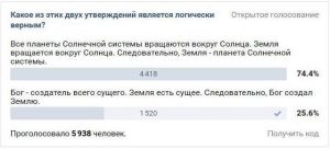
    implicationI've seen this question or variations of it pop up as "provocative" posts in social networks several times. At times they might invite lengthy discussions, where the participants would split into camps - some claim that the first statement is true, because Earth is indeed a planet of the Solar System and God did not create the Earth. Others would laugh at the stupidity of their opponents and argue that, obviously, only the second statement is correct, because it makes a valid logical implication, while the first one does not.

    Not once, however, have I ever seen a proper formal explanation of what is happening here. And although it is fairly trivial (once you know it), I guess it is worth writing up. The root of the problem here is the difference between implication and provability - something I myself remember struggling a bit to understand when I first had to encounter these notions in a course on mathematical logic years ago.

    Indeed, any textbook on propositional logic will tell you in one of the first chapters that you may write

        \[A \Rightarrow B\]

    to express the statement "A implies B". A chapter or so later you will learn that there is also a possibility to write

        \[A \vdash B\]

    to express a confusingly similar statement, that "B is provable from A". To confirm your confusion, another chapter down the road you should discover, that A \Rightarrow B is the same as \vdash A \Rightarrow B, which, in turn, is logically equivalent to A \vdash B. Therefore, indeed, whenever A \Rightarrow B is true, A \vdash B is true, and vice-versa. Is there a difference between \vdash and \Rightarrow then, and why do we need the two different symbols at all? The "provocative" question above provides an opportunity to illustrate this.

    The spoken language is rather informal, and there can be several ways of formally interpreting the same statement. Both statements in the puzzle are given in the form "A, B, consequently C". Here are at least four different ways to put them formally, which make the two statements true or false in different ways.

    The Pure Logic Interpretation

    Anyone who has enough experience solving logic puzzles would know that both statements should be interpreted as abstract claims about provability (i.e. deducibility):

        \[A, B \vdash C.\]

    As mentioned above, this is equivalent to

        \[(A\,\&\, B) \Rightarrow C.\]

    or

        \[\vdash (A\,\&\, B) \Rightarrow C.\]

    In this interpretation the first statement is wrong and the second is a correct implication.

    The Pragmatic Interpretation

    People who have less experience with math puzzles would often assume that they should not exclude their common sense knowledge from the task. The corresponding formal statement of the problem then becomes the following:

        \[[\text{common knowledge}] \vdash (A\,\&\, B) \Rightarrow C.\]

    In this case both statements become true. The first one is true simply because the consequent C is true on its own, given common knowledge (the Earth is indeed a planet) - the antecedents and provability do not play any role at all. The second is true because it is a valid reasoning, independently of the common knowledge.

    This type of interpretation is used in rhetorical phrases like "If this is true, I am a Dutchman".

    The Overly Strict Interpretation

    Some people may prefer to believe that a logical statement should only be deemed correct if every single part of it is true and logically valid. The two claims must then be interpreted as follows:

        \[([\text{common}] \vdash A)\,\&\, ([\text{common}] \vdash B)\,\&\, (A, B\vdash C).\]

    Here the issue of provability is combined with the question about the truthfulness of the facts used. Both statements are false - the first fails on logic, and the second on facts (assuming that God creating the Earth is not part of common knowledge).

    The Oversimplified Interpretation

    Finally, people very unfamiliar with strict logic would sometimes tend to ignore the words "consequently", "therefore" or "then", interpreting them as a kind of an extended synonym for "and". In their minds the two statements could be regarded as follows:

        \[[\text{common}] \vdash A\,\&\, B\,\&\, C.\]

    From this perspective, the first statement becomes true and the second (again, assuming the aspects of creation are not commonly known) is false.

    Although the author of the original question most probably did really assume the "pure logic" interpretation, as is customary for such puzzles, note how much leeway there can be when converting a seemingly simple phrase in English to a formal statement. In particular, observe that questions about provability, where you deliberately have to abstain from relying on common knowledge, may be different from questions about facts and implications, where common sense may (or must) be assumed and you can sometimes skip the whole "reasoning" part if you know the consequent is true anyway.

    Here is an quiz question to check whether you understood what I meant to explain.

    "The sky is blue, and therefore the Earth is round." True or false?

    Tags: , , , ,

  • Posted by Konstantin 07.03.2017 No Comments

    Ever since the "Prior Confusion" post I was planning to formulate one of its paragraphs as the following abstract puzzle, but somehow it took me 8 years to write it up.

    According to fictional statistical studies, the following is known about a fictional chronic disease "statistite":

    1. About 30% of people in the world have statistite.
    2. About 35% of men in the world have it.
    3. In Estonia, 20% of people have statistite.
    4. Out of people younger than 20 years, just 5% have the disease.
    5. A recent study of a random sample of visitors to the Central Hospital demonstrated that 40% of them suffer from statistite.

    Mart, a 19-year Estonian male medical student is standing in the foyer of the Central Hospital, reading these facts from an information sheet and wondering: what are his current chances of having statistite? How should he model himself: should he consider himself as primarily "an average man", "a typical Estonian", "just a young person", or "an average visitor of the hospital"? Could he combine the different aspects of his personality to make better use of the available information? How? In general, what would be the best possible probability estimate, given the data?

    Tags: , , , , , , ,

  • Posted by Konstantin 25.02.2013 No Comments

    If anyone tells you he or she understands probability theory, do not believe them. That person simply does not know enough of it to admit, that probability theory is riddled with paradoxes, where common sense must step aside and wait in silence, or your brain will hurt. Substring statistics is probably among the lesser-known, yet magically unintuitive examples.

    Consider a sequence of random coin flips. Each coin flip is either a "heads" or a "tails", hence the sequence might written down as a sequence of H and T-s: HTHTHHTT...

    It is easy to show that the probability of the sequence to begin with, say, HHH is equal to P(HHH) = 1/8th, as is the case with any other three-letter combination: P(HHT) = P(THH) = P(THT) = 1/8, etc. Moreover, by symmetry, the probability of seeing a particular three-letter combination at any fixed position in the sequence is still always 1/8-th. All three-letter substrings seem to be equivalent here.

    But let us now play a game, where we throw a coin until we see a particular three-letter combination. To be more specific, let us wait until either HHT or HHH comes up. Suppose I win in the first case and you win in the second one. Obviously, the game first proceeds until two heads are flipped. Then, whichever coin flip comes up next determines the winner. Sounds pretty fair, doesn't it? Well, it turns out that, surprisingly, if you count carefully the expected number of coin flips to obtain HHT, it happens to be 8, whereas for HHH it is 14! Ha! Does it mean I have an advantage? Suprisingly again, no. The probability of HHT occuring before HHH in any given sequence is still precisely 0.5 and, as we reasoned initially, the game is still fair.

    We can, however, construct even more curious situations with four-letter combinations. Suppose I bet on HTHT and you bet on THTT.  The expected number of coin flips to obtain my combination can be computed to be 20. The expected number of flips to get your combination is smaller: 18 flips. However, it is still more probable (64%) that my combination will happen before yours!

    If this is not amusing enough, suppose that four of us are playing such a game. Player A bets on the string THH, Player B bets on HHT, player C on HTT and player D on TTH. It turns out that A's combination will occur earlier than B's with probability 75%. B's combination, however, wins over C's with probability 66.7%. C's combination, though, wins over D's with probability 75%. And, to close the loop, D wins over A with probability 66.7%! This is just like the nontransitive dice.

    Hopefully, you are amazed enough at this point to require an explanation for how this all might happen. Let me leave it to you as a small puzzle:

    • Explain in simple terms, how can it happen so that the expected time to first occurrence of otherwise equiprobable substrings may be different?
    • Explain in simple terms, how can it be so that one substring has higher than 50% chance of occuring earlier than some other substring.
    • Finally, explain why the two effects above are not strictly related to each other.

    PS: The theory used to compute actual probabilities and expected times to occurrence of a substring is elegant yet somewhat involved. For the practically-minded, here is the code to check the calculations.

    Tags: , , , ,

  • Posted by Konstantin 07.06.2012 33 Comments

    The following text will only make sense to you if you know the technical details of Support Vector Machine learning.

    Having recently had to give some lectures (1,2,3,4) and exercise sessions (1,2,3,4) on linear classification in a machine learning course, I discovered that one of the most famous linear classification methods, the classical Support Vector Machine, does not seem to be fully specified in any of the prominent reference materials. Namely, the SVM learning procedure produces two parameters: the coefficient vector \bf\alpha and the bias term b. While the problem of finding \bf\alpha is typically explained in sufficient detail, the procedure of computing b is usually swept under the carpet.

    Here is, for example, what we see in the Vapnik's seminal work, the birthplace of SVMs (Section 10.2, page 411):

    Vapnik (page 411)According to my calculations this is plain incorrect, because the corresponding Kuhn-Tucker conditions (in the "soft margin" SVM that we are considering here) are actually:

        \[\alpha_t^0\left(\frac{1}{\gamma}\sum_{i=1}^\ell \alpha_i^0y_i(x_t * x_i) + b-1+\xi_i\right) = 0\]

    The important difference is the presence of the \xi_i term, which is unknown, hence the equation is not useful for finding b. Later on, the reader is also presented with the following summarizing description of the algorithm:

    Vapnik (page 425)Do you see any mention of the way to compute b? I would expect the author to be somewhat more helpful with respect to this detail, which is obviously important for anyone willing to implement their own version of SVM.

    OK, that was an old book, let's take a look at some newer materials. The two books which could be regarded as authoritative sources on the subject of SVMs are probably "An Introduction to Support Vector Machines" and "Kernel Methods for Pattern Analysis". Here is what the first book tells us about computing b (Proposition 6.11, page 106):

    Cristianini (page 106)

    This suggests that in order to compute b we need to find \alpha_i^*, such that C>\alpha_i^*>0, i.e. there must exist at least one training point lying exactly on the margin. Although in most practical situations such support vectors will indeed exist, it is also theoretically possible that there won't be any, i.e. not a single support vector will lie exactly on the margin. Thus, for purposes of implementing SVMs, the provided specification is incomplete.

    The same problem is present in the second book:

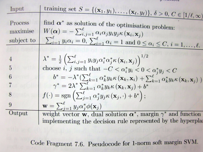
    Shawe-Taylor

    Take a careful look at lines 5-6, which claim that in order to compute b we need to choose i,j such that the corresponding \alpha_i, \alpha_j are strictly between 0 and C. This is not necessarily true for any \alpha_i.

    So then, what is the proper, fully general way of computing b? Of course, it is not too hard to derive, and thus makes for a great course homework exercise (e.g. Exercise 4 here). If you managed to read up to this point, I presume you should be motivated enough to try solving it. If you give up, you are welcome to consult my sample solution (Exercise 4, page 7).

    Tags: , , ,

  • Posted by Konstantin 16.01.2012 No Comments

    This post presumes you are familiar with PCA.

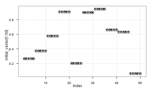
    Consider the following experiment. First we generate a random vector (signal) as a sequence of random 5-element repeats. That is, something like

    (0.5, 0.5, 0.5, 0.5, 0.5,   0.9, 0.9, 0,9, 0.9, 0,9,   0.2, 0.2, 0.2, 0.2, 0.2,   ... etc ... )

    In R we could generate it like that:

    num_steps = 50
    step_length = 5;
    initial_vector = c();
    for (i in 1:num_steps) {
      initial_vector = c(initial_vector, rep(runif(1), step_length));
    }

    Here's a visual depiction of a possible resulting vector:

    Initial random vector

    plot(initial_vector), zoomed in

    Next, we shall create a dataset, where each element will be a randomly shifted copy of this vector:

    library(magic) # Necessary for the shift() function
    dataset = c()
    for (i in 1:1000) {
      shift_by = floor(runif(1)*num_steps*step_length) # Pick a random shift
      new_instance = shift(initial_vector, shift_by)   # Generate a shifted instance
      dataset = rbind(dataset, new_instance);          # Append to data
    }

    Finally, let's apply Principal Component Analysis to this dataset:

    pca = prcomp(dataset)

    Question - how do the top principal components look like? Guess first, then read below for the correct answer.

    Read more...

    Tags: , ,

  • Posted by Konstantin 21.11.2009 No Comments

    In the recent weeks I had to give a few introductory lectures on supervised machine learning within Jaak's data mining course. I also provided the students some home assignments, and there it was especially tricky to find a simple, fun and discussable exercise, which might help to form some intuition regarding the inherent difficulties of learning from data such as overfitting, multiple testing, and the like. The following is what I came up with and I find it a rather successful creation. It is remarkable that of the 80 students participating in the course only 4 or so came up with the correct answer 🙂

    The Riddle

    After the lecture on supervised machine learning at the University of Mordor, the teacher, Sauron, gave the students a dataset of the following form:

                1) ABACDAFXYZ    -> good
                2) CEGXEAELWMN   -> good
                3) NUWAB         -> bad
                        ...
               20) QRELAZMNPCXA  -> good

    The inputs were seemingly arbitrary strings of latin characters: these were the terrible spells known only to Sauron and chosen by Sauron at random from his Great Book of Terrible Spells. The output was a binary variable, classifying each spell as good or bad. There were 20 observations in total in the dataset.

    The students were given a task: on the basis of this data, come up with a generic spell classifier. Sauron promised to test their result on the next lecture as follows: he will pick another random terrible spell from the book and require each student to make a prediction. The student whose prediction is wrong will have to jump down from the tower as a punishment.

    The first student, Aghargh, who happened to be slacking on the lecture, couldn't come up with any smart ways to solve the task, so he ended up just counting the proportion of "good" and "bad" spells in the dataset. Having observed that 16 of the 20 spells were "good", he decided to predict "good" when asked.

    The second student, Bughrorc, chose a smarter way. Firstly, he converted each string into a vector of binary attributes — one attribute for each letter, having value "1" if that letter was present in the corresponding spell and "0" otherwise. He then split the data randomly into a training set (15 instances) and a test set (5 instances), and attempted training various classifiers using the MordorMiner software. After some experimenting he finally found five classifiers that could predict all of the training examples correctly. One of these also predicted all of the testing examples correctly. He decided to use this classifier on the forthcoming test.

    On the day of testing, Sauron asked the students to classify the spell YOZAZA. Aghargh, as he decided, provided the answer "good". Bughrorc's classifier analyzed the string and claimed that the answer should be "bad"

    Which of the students, do you think, might have a better chance of not jumping from the tower? Why? Can you quantify your answer?

    Tags: , , ,

  • Posted by Konstantin 28.01.2009 5 Comments

    Imagine that you have just derived a novel IQ test. You have established that for a given person the test produces a normally-distributed unbiased estimate of her IQ with variance 102. That is, if, for example, a person has true IQ=120, the test will result in a value from a N(120,102) distribution. Also, from your previous experiments you know that among all the people, IQ has a N(110,152) distribution.

    One a sunny Monday morning you went out on a street and requested the first bypasser (whose name turned out to be John) to take your test. The resulting score was t=125. The question is: what can you conclude now about the true IQ of that person (assuming, of course, that there is such a thing as a "true IQ"). There are at least two reasonable approaches to this problem.

    1. You could apply the method of maximum likelihood. Here's John, standing beside you, and you know his true IQ must be some real number a. The test produced an unbiased estimate of a equal to 125. The likelihood of the data (i.e. the probability of obtaining a test score of 125 for a given a) is therefore:

          \[P[T=125|A=a]=\frac{1}{\sqrt{2\pi 10^2}}\exp\left(-\frac{1}{2}\frac{(125-a)^2}{10^2}\right)\]

      The maximum likelihood method suggests picking the value of a that maximizes the above expression. Finding the maximum is rather easy here and it turns out to be at a=125, which is pretty natural. You thus conclude that the best what you can say about John's true IQ is that it is approximately 125.

    2. An alternative way of thinking is to use the method of maximum a-posteriori probability, where instead of maximizing likelihood P[T=125|A=a], you maximize the a-posteriori probability P[A=a|T=125]. The corresponding expression is:

       \begin{multiline} P[A=a|T=125] \sim P[T=125|A=a]\cdot P[A=a] = \\ = \frac{1}{\sqrt{2\pi 10^2}}\exp\left(-\frac{1}{2}\frac{(125-a)^2}{10^2}\right)\cdot \frac{1}{\sqrt{2\pi 15^2}}\exp\left(-\frac{1}{2}\frac{(110-a)^2}{15^2}\right) \end{multiline}

      Finding the required maximum is easy again, and the solution turns out to be a=120.38. Therefore, by this logic, John's IQ should be considered to be somewhat lower than what the test indicates.

    Which of the two approaches is better? It might seem utterly unbelievable, but the estimate provided by the second method is, in fact, closer to the truth. The straightforward "125", proposed to by the first method is biased, in the sense that on average this estimate is slightly exaggerated. Think how especially unintuitive this result is from the point of view of John himself. Clearly, his own "true IQ" is something fixed. Why on Earth should he consider "other people" and take into account the overall IQ distribution just to interpret his own result obtained from an unbiased test?

    To finally confuse things, let us say that John got unhappy with the result and returned to you to perform a second test. Although it is probably impossible to perform any real IQ test twice and get independent results, let us imagine that your test can indeed be repeated. The second test, again, resulted in a score of 125. What IQ estimate would you suggest now? On one hand, John himself came to you and this time you could regard his IQ as a "real" constant, right? But on the other hand, John is just a person randomly picked from the street, who happened to take your test twice. Go figure.

    PS: Some additional remarks are appropriate here:

    • Although I'm not a fan of The Great Frequentist-Bayesian War, I cannot but note that the answer is probably easier if John is a Bayesian at heart, because in this case it is natural for him to regard "unknown constants" as probability distributions and consider prior information in making inferences.
    • If it is hard for you to accept the logic in the presented situation (as it is for me), some reflection on the similar, but less complicated false positive paradox might help to relieve your mind.
    • In general, the correct way to obtain the true unbiased estimate is to compute the mean over the posterior distribution:

          \[E[a|T=125] = \int a \mathrm{dP}[a|T=125]\]

      In our case, however, the posterior is symmetric and therefore the mean coincides with the maximum. Computing the mean by direct integration would be much more complicated.

    Tags: , , , ,

  • Posted by Konstantin 15.01.2009 21 Comments

    Consider the following excerpt from a recent article in the British Medical Journal:

    Puzzle

    Mike has only two children, and they are called Pat and Alex, which could equally be boys’ or girls’ names. In fact, Pat is a girl. What is the probability that Alex is a boy?

    a 50%
    b Slightly less than 50%
    c Slightly more than 50%
    d Between 60% and 70%
    e Between 40% and 30%

    d—Although this could be about the relative popularity of ambiguous names for boys and girls or about subtle imbalances in the sex ratio, it is not meant to be. The clue to the correct answer is in thinking about what we do not know about the family and what we do know already, and applying this to the expected probabilities of girls and boys.

    We do not know if Pat was born first or second. We do know that there are only two children and that Pat is a girl. I am assuming that in the population, 50% of children are girls.

    The birth order and relative frequency of two child families are: boy, boy (25%), girl, girl (25%), boy, girl (25%) girl, boy (25%). We know Mike’s family does not have two boys, since Pat is a girl, so we are only left with three choices for families with at least one girl. Two of these pairs have a boy and one does not. Hence the probability that Alex is a boy is two thirds or 66.7%.

    If we had been told that Pat was born first then the probability that Alex is a boy drops to 50%.

    The well-known "Boy or Girl" paradox that is referenced in the fragment above is probably as old as the probability theory itself. And it is therefore quite amusing to see an incorrect explanation for it presented in a serious journal article. You are welcome to figure out the mistake yourself.

    For completeness sake, here is my favourite way of presenting this puzzle:

    In the following, let Mike be a randomly chosen father of two kids.

    1. Mike has two kids, one of them is a boy. What is the probability that the other one is a girl?
    2. Mike has two kids, the elder one is a boy. What is the probability that the other one is a girl?
    3. Mike has two kids. One of them is a boy named John. What is the probability that the other one is a girl?
    4. I came to visit Mike. One of his two kids, a boy, opened the door to me. What is the probability that Mike's other child is a girl?
    5. I have a brother. What is the probability that I am a girl?
    6. I have a brother named John. What is the probability that I am a girl?

    You can assume that boys and girls are equiprobable, the births of two kids are independent events, a randomly chosen boy will be named John with probability p, and that a family may have two kids with the same name.

    If you haven't tried solving these yet, give it a try. I'm pretty sure you won't do all 6 questions correctly on the first shot.

    Tags: , , ,