• Posted by Konstantin 04.12.2011 1 Comment

    There is one rule of thumb that I find quite useful and happen to use fairly often. It is probably not widely known nor described in textbooks (I stumbled upon it on my own), so I regularly have to explain it.  Next time I'll just point out to this post.

    The rule is the following: a proportion estimate obtained on a sample of n points should only be trusted up to an error of \frac{1}{\sqrt{n}}.

    For example, suppose that you read in the newspaper that "25% of students like statistics". Now, if this result has been obtained from a survey of 64 participants, you should actually interpret the answer as 0.25\pm\frac{1}{\sqrt{64}}, that is, 0.25\pm 0.125, which means that the actual percentage lies somewhere between 12.5% and 37.5%.

    As another example, in machine learning, you often get to see cases where someone evaluates two classification algorithms on a test set of, say, 400 instances, measures that the first algorithm has an accuracy of 90%, the second an accuracy of, say, 92%, and boldly claims the dominance of the second algorithm. At this point, without going deeply into statistics, it is easy to figure that 1/\sqrt{400} should be somewhere around 5%, hence the difference between 90% and 92% is not too significant to celebrate.

    The Explanation

    The derivation of the rule is fairly straightforward. Consider a Bernoulli-distributed random variable with parameter p. We then take an i.i.d. sample of size n, and use it to estimate \hat p:

        \[\hat p = \frac{1}{n}\sum_i X_i\]

    The 95% confidence interval for this estimate, computed using the normal approximation is then:

        \[\hat p \pm 1.96\sqrt{\frac{p(1-p)}{n}}\]

    What remains is to note that 1.96\approx 2 and that \sqrt{p(1-p)} \leq 0.5. By substituting those two approximations we immediately get that the interval is at most

        \[\hat p \pm \frac{1}{\sqrt{n}}\]

    Limitations

    It is important to understand the limitations of the rule. In the cases where the true proportion estimate is p=0.5 and n is large enough for the normal approximation to make sense (20 is already good), the one-over-square-root-of-n rule is very close to a true 95% confidence interval.

    When the true proportion estimate is closer to 0 or 1, however, \sqrt{p(1-p)} is not close to 0.5 anymore, and the rule of thumb results in a conservatively large interval.

    In particular, the true 95% confidence interval for p=0.9 will be nearly two times smaller (\approx 0.6/\sqrt{n}). For p=0.99 the actual interval is five times smaller (\approx 0.2/\sqrt{n}). However, given the simplicity of the rule, the fact that the true p is rarely so close to 1, and the idea that it never hurts to be slightly conservative in statistical estimates, I'd say the one-over-a-square-root-of-n rule is a practically useful tool in most situations.

    Use in Machine Learning

    The rule is quite useful to quickly interpret performance indicators of machine learning models, such as precision, accuracy or recall, however, you should make sure you understand what proportion is actually being computed for each metric. Suppose we are evaluating a machine learning model on a test set of 10000 elements, 400 of which were classified as "positive" by the model. We measure the accuracy of the model by computing a proportion of correct predictions on the whole set of 10000 elements. Thus, the n here is 10000 and we should expect the confidence intervals of the resulting value to be under 1 percent point. However, the precision of the model is measured by computing the proportion of correct predictions among the 400 positives. Here n is actually 400 and the confidence intervals will be around 0.05.

    The rule can also be used to choose the size of the test set for your model. Despite the popular tradition, using a fraction of your full dataset for testing (e.g. "75%/25% split") is arbitrary and misguided. Instead, it is the absolute size of the test sample that you should care most about. For example, if you are happy with your precision estimates to be within a 1% range, you only need to make sure your test set would include around 10000 positives. Wasting an extra million examples for this estimate will increase the quality of your estimate, but you might be better off leaving these examples for model training instead.

    Tags: , ,

  • Posted by Konstantin 12.02.2010 4 Comments

    Statistics is mainly about using the observed data to make conclusions about the "real state of affairs", underlying that data. A classical and most widely spread technique for making these conclusions is based on significance testing. In simple terms, the idea of significance testing is to ask the question: "if the real state of affairs were X, how probable would it be for us to obtain the data D we are currently observing?". If the answer is "rather unprobable" (e.g. p < 0.05), the common decision is to reject the proposition X in favor of the alternative "not X". Otherwise the researcher claims to "see no reason to reject X".

    The logic behind that reasoning seems quite solid from the first glance, yet it is well known to be faulty. Naturally, the fact that the likelihood of the data P(D | X) is low need not imply that the underlying hypothesis is wrong - it might very well be the case that the data by itself is already rare enough to make this value low. The only correct way of making sound judgments is to consider the a-posteriori probability of the hypothesis P(X | D) instead. However, the latter can be quite inconvenient to compute. Besides, the wild popularity of significance tests and p-values seems to indicate that the issue is not at all that serious. Really, P(X | D) looks so similar to P(D | X), who cares?

    Book cover

    The book "What If There Were No Significance Tests?", which I stumbled upon recently while browsing a stray library shelf, makes it clear that this issue is not a joke. It is a collection of chapters written by renowned statisticians (most of which some-why work in the field of psychology), that quite convincingly condemns the widespread overuse of p-values and the related significance-based hypothesis testing in favor of other approaches. The main point is nailed quite precisely in the very first essay by Jacob Cohen, which I strongly advise you to read right now in order to get rid of any illusions you might still have regarding significance testing. And when you're done with that, you can continue reading this post.

    In the following I shall provide my personal summary of the marvelous "Member of Congress" example from J.Cohen's essay. So far it is the best illustration I know of, about why exactly it is dangerous to use significance tests blindly.

    Improbable does not mean impossible

    Consider the following situation. We have observed a person which we know to be a Member of the US Congress. We are interested in testing the hypothesis, that this person is an American citizen. To apply the significance testing methodology, we proceed by estimating the p-value:

    P(Congressman | American) ~ 535/300 000 000.

    This is clearly below the popular 0.05 threshold. As a result, we are forced to reject the null-hypothesis and conclude that the person is not an American citizen. Bummer.

    What is the problem here? Well, one thing is worth noting - while the probability for an American to be a congressman is low, it is even lower (precisely, zero), for a non-American. So maybe we would have been better off if we expanded the procedure above to the following "maximum-likelihood"-style reasoning:

    Considering that the likelihood P(Congressman | American) is greater than the likelihood P(Congressman | non-American), we must conclude that the person in front of us is an American rather than not.

    Did we just solve the problem? Is it enough to consider "p-values both ways" to clear things up? No!

    Maximum likelihood does not work

    Let us now consider a reversed situation. We are faced with a person, which, we know, is an American. We are interested in the hypothesis that he is a congressman. Compute the two likelihoods:

    P(American | Congressman) = 1

    P(American | not Congressman) ~ 300 000 000 / 6 700 000 000

    Observing that the first likelihood is greater than the second we are forced to conclude that the person in front of us is indeed a congressman. Bummer, again!

    Only by multiplying the likelihood with the marginal probability P(Congressman) could we have obtained the correct decision. Which is, to say, we must have been estimating the probabilities the other way around from the start.

    To summarize, be wary of these pitfalls. I would not agree with the strong negative opinion of the authors of the book, though. After all, a lot of stuff is quite fruitfully done nowadays using p-values only. However, each time you use them, do it sensibly and keep in mind the following two aspects:

    1. If your p-value is low, can this be solely due to low marginal probability of the data? What is the "reversed" p-value? What is the power of your test?
    2. If you suspect that your hypotheses might be subject to a highly non-uniform prior probabilities, do not use bare p-values. You must consider the prior!

    Tags: , ,

  • Posted by Margus 25.10.2009 5 Comments

    That is, if we are lucky and everything is done according to the proper tradition of doing statistics with 1% confidence intervals. In practice, things are probably even worse (many use 5% for instance), but this is what you would expect when everyone used proper methodology.

    Think about it...

    Tags: , ,

  • Posted by Konstantin 11.10.2009 2 Comments

    I've recently stumbled upon a simple observation, which does not seem to be common knowledge and yet looks quite enlightening. Namely: polynomials provide an excellent way of modeling data in an order-agnostic manner.

    The situations when you need to represent data in an order-agnostic way are actually fairly common.  Suppose that you are given a traditional sample x_1, x_2, \dots, x_n and are faced with a task of devising a generic function of the sample, which could only depend on the values in the sample, but not on the ordering of these values. Alternatively, you might need to prove that a given statistic is constant with respect to all permutations of the sample. Finally, you might simply wish to have a convenient mapping for your feature vectors that would lose the ordering information, but nothing else.

    The most common way of addressing this problem is sorting the sample and working with the order statistics x_{(1)}, x_{(2)}, \dots, x_{(n)} instead of the original values. This is not always convenient. Firstly, the mapping of the original sample to the corresponding vector of order statistics (i.e. the sorting operation) is quite complicated to express mathematically. Secondly, the condition that the vector of order statistics is always sorted is not very pleasant to work with. A much better idea is to represent your data as a polynomial of the form

        \[p_x(z) = (z+x_1)(z+x_2)\dots(z+x_n)\,.\]

    This will immediately provide you with a marvellous tool: two polynomials p_x and p_y are equal if and only if their roots are equal, which means, in our case, that the samples x_1,\dots,x_n and y_1,\dots,y_n are equal up to a reordering.

    Now in order to actually represent the polynomial we can either directly compute its coefficients

        \[p_x(z) = z^n + a_1z^{n-1} + \dots + a_n\,,\]

    or calculate its values at any n different points (e.g. at 0,1,\dots,n-1) - in any case we end up with the same amount of data as we had originally (i.e. n values), but the new representation is order-agnostic and has, arguably, much nicer properties than the order statistics vector.

    It is not without its own problems, of course. Firstly, it requires at least \Omega(n^2) time to compute. Secondly, not every polynomial will have n real-valued roots. And thirdly, the interpretation of the new "feature vector" is not necessarily intuitive or meaningful. Yet nonetheless, it's a trick to consider.

    Tags: , , , ,

  • Posted by Swen 25.08.2009 No Comments

    There seems to be a wide split of opinions between theoreticians and practitioners. Namely, some theoreticians define pseudorandomness in terms of complexity theory. As a result, the corresponding constructions are inherently slow and thus rejected by practitioners. This short blog post tries to address some common misconceptions.

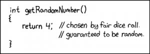
    Random number generator by xkcd

    A random number generator by xkcd

    Formally, a pseudorandom generator is a deterministic function f:\mathcal{S}\to\mathcal{R} which takes a (relatively short) seed s and converts it into an element of \mathcal{R}. In most cases, we as computer scientists are interested in functions f:\{0,1\}^n\to\{0,1\}^\ell. However, there are other reasonable domains, too. For instance, when performing Monte-Carlo integration in the region [0,1], we would be interested in the functions of type f:\{0,1\}^n\to[0,1]^\ell.

    It is important to note that any function of type f:\mathcal{S}\to\mathcal{R} is a pseudorandom generator. However, not all of those functions are equally good for all purposes. There are two main properties that are used to discriminate between various pseudorandom functions. First, we can talk about the efficiency of a pseudorandom generator, i.e., how fast can we compute f(s). Second, we can talk about the statistical properties of the output f(s).

    Before going into the details, let us establish why anyone should use pseudorandom generators at all. There is an interesting controversy in the computer science, as well in statistics. Many algorithms assume that it is possible to use uniformly distributed numbers. For example, Monte-Carlo integration is based on the law of large numbers:

        \[\Pr[\lim_n\frac{1}{N}\sum_{i=1}^N g(x_i)=\int_0^1g(x)dx] = 1\]

    whenever x_1,\ldots,x_N are taken independently and uniformly from the range [0,1]. Similarly, one can provide theoretical bounds for the randomized version of quicksort, provided that we can draw elements uniformly from a set \{1,\ldots,K\}. However, computers are mostly made of deterministic parts and it turns out to be really difficult to automatically collect uniformly distributed bits. A design of a device that would solve this problem is far from trivial.

    The first official solution to this problem was posed in 1927 when a student of Karl Pearson published a table of random numbers. Later such tables were built by the RAND Corporation. That is, the function f was explicitly specified through a big table. Of course, such a table is useful only if it can be used as a "reliable" source of random numbers. In particular, the value of

        \[\frac{1}{N}\sum_{i=1}^N g(x_i)\]

    should be as close to \int_0^1 g(x)dx as possible. Since there are infinite number of functions, we cannot actually check this condition. Instead, statisticians performed a series of tests on the table to verify that the sequence x_1,x_2,\ldots looks as close to random as possible.  If we extend this concept properly, we get the modern quantification of pseudorandomness.

    Formally, a function f:\mathcal{S}\to\mathcal{R} is a (t,\varepsilon)-secure pseudorandom generator if for any t-time algorithm A:

        \[|\Pr [r\gets\mathcal{R}: A(r)=1]-\Pr[s\gets\mathcal{S}: A(f(s))=1]|\leq \varepsilon\]

    where the probabilities are taken over the uniform choices of s and r. In more intuitive terms, if you replace the randomness r with f(s) and your algorithm runs in time t, then the switch generates no easily observable discrepancies.

    As an illustrative example, consider a probabilistic combinatorial search algorithm B that runs in time t_1 and outputs a solution that can be verified in time t_2. In this case, the use of a (t_1+t_2,\varepsilon) -secure pseudorandom generator within B instead of pure randomness would decrease the probability of B finding a solution by at most \varepsilon. Indeed, otherwise we could construct a (t_1+t_2)-time algorithm C that outputs 1, if B finds the solution and 0 otherwise, and use it to discern the pseudorandom generator from true randomness with success at least \varepsilon. This would contradict the fact that we have a true (t_1+t_2,\varepsilon) -secure pseudorandom generator.  Similar argument can be proven also for the Monte-Carlo integration algorithm. Note that parameters t and \epsilon can be arbitrary real numbers. For the combinatorial search algorithm that takes 3 weeks CPU time, you might use a (3\ \text{week}, 0.01)-secure pseudorandom generator.

    There are essentially two reasonable complaints about the pseudorandom generators. First, since obtaining random bits is hard, we have not solved the problem completely, as we must still get the seed from somewhere. This is indeed a valid problem. For instance, the standard rand() function in C is known to fail the NIST statistical test and thus you might actually observe inconsistencies when using rand() directly or generating a seed for a more complex function with rand(). The latter does not mean that rand() is not a pseudorandom generator, rather that its quality might be low for certain applications. As a complete solution, you would like to get a function f:\{1\}\to\mathcal{R}. For some tasks, such as Monte-Carlo integration of certain functions the corresponding solution is known (see multidimensional integration and sparse grids).

    However, we still do not know how to do it in general, i.e., how to convert randomized algorithms into deterministic ones without significant losses in their performance. The corresponding area of research is known as derandomization. Second, one might argue that we could prove directly that by replacing r with f(s), the performance of the algorithm does not deteriorate much. However, this is not an easy task and it is usually not a valid option for usual mortals.

    To summarize, whenever you use a certain function f to extend a random seed in your implementation you actually have to believe that it does not affect performance, i.e., f is a pseudorandom generator with appropriate (t,\varepsilon) parameter values. Whether you should use f(x)=1, rand() in C, or something more elaborate, depends on the application.

    Tags: , , ,

  • Posted by Konstantin 11.08.2009 7 Comments

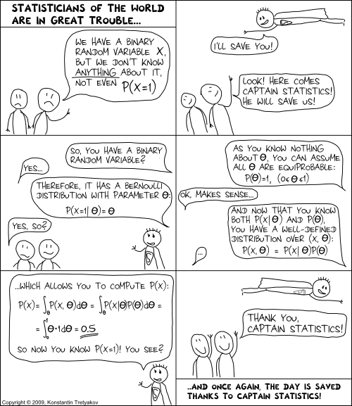
    Inspired by Swen

    Tags: , , ,

  • Posted by Konstantin 26.03.2009 No Comments

    Symbols and Reality

    Mathematics is a language. An abstract set of generic symbols for describing concepts, objects and systems. Take, for example, the symbol "5", "five". What is it? Is it a real-world object? No. It is just a symbol. You are free to attach to it any interpretation that you deem appropriate. Of course, most of the times you would use the common interpretation of "5" as a natural number, denoting, well, "five of something". Literally meaning that you can count something as "this, this, this, this and this".

    Take a moment to reflect on the degree of generality of this simple concept, "five". It can be applied to practically anything. Five apples, five centimeters, five centuries are notions as different from each other as you could imagine, and yet all of them relate to the concept "five". On the other hand, it is not too generic to be useless: "five" is radically different from "six", "seven", and an infinity of other numbers. This kind of magical balance between generality and specificity is common to mathematics. This is what makes mathematics both widely applicable and yet still incredibly useful.

    Besides just giving us symbols like 5 or 6, mathematics provides an endless variety of ways for expressing "rules", "operations", "statements", "derivations", "computations" and the like, such as 5+5=10, or \forall x:\, x^2 - 10x \gt -5^2, etc. Once again, all of these rules, operations and statements need not necessarily bear any relation with reality. After all, they all are just a cunning play with symbols. And yet, quite often they do describe reality incredibly well. I know that 512 apples and 512 apples will make 1024 apples together. How do I know it? Certainly not because I checked it on real apples! I just believe that the real-world operation of "adding apples" can be satisfactory modeled using the formal symbolic framework of natural numbers and the operation of addition on them. Why do I believe it? This is a tricky philosophical question that we shall leave aside for now. But remember that any application of mathematics to the real world is always based on a belief that the chosen model describes the world well.

    The Nature of Uncertainty

    There are often cases where we would like to use mathematics to model "uncertainty". Now remember that from the point of view of pure math there are no such things as inherent "certainty" and "uncertainty". Mathematics will always operate on symbols and use precise, uniquely reproducible transformation rules between these symbols. Yet there are often cases when we, in our interpretations of these symbols, would like refer to certain entities as "uncertain". The reasons can be various:

    1. Sometimes, we would like to use a single generalized concept to summarize multiple objects.
      - What is the height of a human?

      There is no single clear answer and yet it is possible to provide one using an uncertainty model such as a probability distribution.
    2. Sometimes, we want to reason about some single numeric value which, even if it were well-defined, we just could not compute exactly.
      - What is the AVERAGE height of a human?

      In theory, it is a number you could measure by lining up all the people in the world and computing their average, but it is certainly an infeasible project.
    3. Sometimes, the notion we would like to reason about is inherently not well-defined.
      - What is MY height, after all?

      The answer depends on a number of factors such as time, measuring equipment, my precise posture, etc. Instead of taking all of these into consideration, we prefer to exploit an uncertainty model.
    4. Sometimes we just need a single concept to encapsulate a state of knowledge more sophisticated than pure numeric equality. For example, to express the fact like "my height IS GREATER THAN 150cm" without using the "greater than" operation.

    There are also other situations, which are difficult to classify, but in all cases the idea is the same — for one reason or another we "don't know" (or "don't specify") the exact single quantity we want to reason about, an yet we still "know something" about it. In fact, amusingly, the amount of information that we use to represent an "uncertain" quantity is often much greater than the amount of information we would need to represent a "certain" one. For example, there are much more probability distributions than there are real numbers. Therefore, picking one probability distribution to represent our knowledge of a number is, in principle, a more informative step than picking a single real number. And yet, we call the former case "uncertainty" and the latter one "certainty". Because that's how we choose to name and interpret things, that's how we believe these concepts relate to reality.

    Models of Uncertainty

    The adjective "uncertain" is something you could, in theory, apply generically to any type of data. In a computer scientist's terms, it makes perfect sense to talk about datatypes "uncertain int", "uncertain real", "uncertain boolean", "uncertain string", "uncertain graph", "uncertain map" and maybe even "uncertain uncertain real" and the like. Let's limit ourselves here to the consideration of uncertain numbers only, as these are the most commonly used and well-studied types of uncertainty. So how do you model (or, say, "implement") "uncertain real"? Here is a short list of the most popular options:

    1. Approximate numbers.Although you might not consider it as a smart approach, this is probably the most common choice in practice — using a usual number to represent an uncertain one. In this case the uncertainty is purely interpretative: instead of stating x = 5 you would, perhaps, write x \approx 5, denoting your state of ignorance. Quite often you would not even care to use the approximate equality sign, presuming it is clear from the context that you are not supposed to provide an ideally exact measurement: — What is your height? — It is 180cm. This works quite well in simple real-life situations, such as buying a kilogram of apples or discussing the horsepowers in a friend's motorbike, but is also applicable to some more technical cases, such as computing the distance to the nearest star.The advantage of such implied uncertainty is that you do not really need to deal with it. All of your familiar arithmetic operations come for free, together with their well established interpretations and the nice properties, theories and theorems. The disadvantage is that once your data is approximate, all of these theories and theorems become approximate too. So, although it could often be acceptable to claim x \approx 5, y \approx 10 \Rightarrow x + y \approx 15, you would have problems explaining more complicated steps, such as "x \approx 5 \Rightarrow f(x) \approx f(5) for a continuous f".But what to do if you need to perform such steps? Consider intervals instead!
    2. Intervals.The second most popular method of representing an uncertain real number is to provide an interval where it falls into. It is ubiquitous in engineering disciplines. Most often an interval is expressed either as x\pm\Delta x or by following the significant figures convention (e.g. writing 180.00 to denote 180±0.01). It is an improvement over the previous approach, because now you have a way to quantify the effect of function application on uncertainty. For example, a commonly used rule would be

      f(x\pm\Delta x) \approx f(x)\pm\left(\frac{\partial f(x)}{\partial x} \Delta x\right),

      where f is a differentiable function.

    3. Sets.An approach slightly more general than the "interval" technique would be to provide a set of values, to which the value of interest could belong to. So, instead of stating x = 5 you could write, for example, x \in \{4,5,7\}.This allows for more mathematical rigour. For example: x \in \{4,5,7\} \Rightarrow f(x) \in \{f(4), f(5), f(7)\}. Moreover, besides the standard algebraic operations, the set representation allows to update the knowledge about an uncertain value easily using set unions and intersections:

      x \in A, x \in B \Rightarrow x \in A\cap B.

      However, sets are "heavy" object to work with, so you don't see this approach being used too often in practical computations. Some Monte-Carlo simulations would use a set to represent approximate solutions, but they would convert it to a probability distribution as soon as possible. This leads us to the next item on the list.

    4. Probability distributions.If the previous methods were either too crude, too ad-hoc or too heavy, then probability theory was designed to provide flexible balance and help overcome most of their drawbacks. To represent a number it suggests us to use a probability measure - an additive function that assigns a weight to each set, which could contain the value of interest. The greater the weight of a set - the more probable it is that the value belongs to that set. By convention, the minimum possible weight of a set is 0, which we usually interpret as "the value almost certainly does not belong to that set", and the maximum weight is 1, with a corresponding interpretation "the value almost certainly belongs there". Representing a function defined on sets is complicated, so usually we use a simpler equivalent representation: a cumulative distribution function (CDF) or a probability density function (PDF). The plot of the latter is especially insightful and provides a nice visual cue about the nature of uncertainty being modeled.It is impossible to enumerate all the virtues of using a probability distribution as an uncertainty model. A probability distribution is a flexible structure, capable of accomodating most "common" kinds of uncertainty. There is an authoritative, well-developed theory and a wide range of both practical and theoretical tools available. Besides the standard algebraic operations, you have rules for updating knowledge (such as the Bayes rule) and a range of facilities for decision making (estimation, hypothesis testing, etc). Finally, there are various interpretations available for you to choose from.Of course, there are potential drawbacks, too. On the practical side, it is not always computationally convenient to work with a probability measure. It is a function, after all, and when specified arbitrarily it can either take too much space to represent or too much time to compute. The use of smoothing and approximation techniques can somewhat relieve the problem, but comes at the price of additional assumptions and simplifications. Secondly, a probability distribution is not capable of representing any kind of uncertainty: for example, there is no probability distribution corresponding to the statement "x < 5". Thirdly, the requirement for a probability density to be normalized to sum to 1 is sometimes inconvenient (because you have to normalize) or unintuitive (because it seems to declare that there is a single uncertain value "hidden inside").

      For example, consider the picture on the right and try to provide a concise description of the set of black pixels on it. This will be an uncertain notion because, well, a gray pixel is also somewhat black, isn't it? And although you could provide a probability distribution of "black" on the picture, you would probably intuitively prefer to assign a "truth-value" between 0 and 1 to each pixel, with 1 corresponding to "certainly black" and 0 to "certainly not black". This would, however, violate the "sum-to-one" normalization rule and thus would not be a probability density. What would it be? A fuzzy set.

    5. Fuzzy sets.A fuzzy set is a set whose elements can have a degree of membership between 0 and 1. It is therefore something inbetween a set (because it "feels" like a set) and a probability density (because it is a function, only this time normalized to have a maximum of 1, instead of the integral of 1). A person familiar with probability theory will also easily recognize a straightforward analogy of a fuzzy set to a likelihood function.Fuzzy sets seem to be a natural uncertainty model in various circumstances, such as the "black pixels" example above. They are often conceptually simpler to specify than probability densities, and lack the interpretation controversy surrounding probability theory. On the other hand, the theory of fuzzy sets is not as extensive as that of probabilities. It is rich in operations like max and min, which makes some things computationally difficult. Besides, the lack of a universal interpretation for fuzzy membership values results in a lack of simple unique decision-making facilities. There are just way too many defuzzification rules to choose from.
    6. ... and more.A variety of other approaches is available, the most important ones being Possibility theory, and Dempster-Shafer theory. However, as this text has already grown too long for a blog post, I shall leave the detailed description of these to Wikipedia.

    Summary

    The main message of this exposition is actually quite simple. There are various approaches to modeling uncertainty. They differ in the type of supported operations and, most importantly, in the way we interpret them and map to the real world entities. But nonetheless, these are all still just methods for modeling uncertainty, each with its own advantages and limitations. Moreover, in most situations, as long as you use the math "reasonably", the models are approximately equivalent in terms of the results and decisions you might end up with using them. That is probably the reason why practitioners would rarely consider anything more sophisticated than a probability measure (except, perhaps, when they are feeling adventurous). And that is why it can sometimes be complicated to promote the more "modern" approaches without the awkward looks from the side of the "traditional statistics". After all, these approaches are competing on the same field with The One and Only, Probability Theory.

    Tags: , , , ,

  • Posted by Konstantin 28.01.2009 5 Comments

    Imagine that you have just derived a novel IQ test. You have established that for a given person the test produces a normally-distributed unbiased estimate of her IQ with variance 102. That is, if, for example, a person has true IQ=120, the test will result in a value from a N(120,102) distribution. Also, from your previous experiments you know that among all the people, IQ has a N(110,152) distribution.

    One a sunny Monday morning you went out on a street and requested the first bypasser (whose name turned out to be John) to take your test. The resulting score was t=125. The question is: what can you conclude now about the true IQ of that person (assuming, of course, that there is such a thing as a "true IQ"). There are at least two reasonable approaches to this problem.

    1. You could apply the method of maximum likelihood. Here's John, standing beside you, and you know his true IQ must be some real number a. The test produced an unbiased estimate of a equal to 125. The likelihood of the data (i.e. the probability of obtaining a test score of 125 for a given a) is therefore:

          \[P[T=125|A=a]=\frac{1}{\sqrt{2\pi 10^2}}\exp\left(-\frac{1}{2}\frac{(125-a)^2}{10^2}\right)\]

      The maximum likelihood method suggests picking the value of a that maximizes the above expression. Finding the maximum is rather easy here and it turns out to be at a=125, which is pretty natural. You thus conclude that the best what you can say about John's true IQ is that it is approximately 125.

    2. An alternative way of thinking is to use the method of maximum a-posteriori probability, where instead of maximizing likelihood P[T=125|A=a], you maximize the a-posteriori probability P[A=a|T=125]. The corresponding expression is:

       \begin{multiline} P[A=a|T=125] \sim P[T=125|A=a]\cdot P[A=a] = \\ = \frac{1}{\sqrt{2\pi 10^2}}\exp\left(-\frac{1}{2}\frac{(125-a)^2}{10^2}\right)\cdot \frac{1}{\sqrt{2\pi 15^2}}\exp\left(-\frac{1}{2}\frac{(110-a)^2}{15^2}\right) \end{multiline}

      Finding the required maximum is easy again, and the solution turns out to be a=120.38. Therefore, by this logic, John's IQ should be considered to be somewhat lower than what the test indicates.

    Which of the two approaches is better? It might seem utterly unbelievable, but the estimate provided by the second method is, in fact, closer to the truth. The straightforward "125", proposed to by the first method is biased, in the sense that on average this estimate is slightly exaggerated. Think how especially unintuitive this result is from the point of view of John himself. Clearly, his own "true IQ" is something fixed. Why on Earth should he consider "other people" and take into account the overall IQ distribution just to interpret his own result obtained from an unbiased test?

    To finally confuse things, let us say that John got unhappy with the result and returned to you to perform a second test. Although it is probably impossible to perform any real IQ test twice and get independent results, let us imagine that your test can indeed be repeated. The second test, again, resulted in a score of 125. What IQ estimate would you suggest now? On one hand, John himself came to you and this time you could regard his IQ as a "real" constant, right? But on the other hand, John is just a person randomly picked from the street, who happened to take your test twice. Go figure.

    PS: Some additional remarks are appropriate here:

    • Although I'm not a fan of The Great Frequentist-Bayesian War, I cannot but note that the answer is probably easier if John is a Bayesian at heart, because in this case it is natural for him to regard "unknown constants" as probability distributions and consider prior information in making inferences.
    • If it is hard for you to accept the logic in the presented situation (as it is for me), some reflection on the similar, but less complicated false positive paradox might help to relieve your mind.
    • In general, the correct way to obtain the true unbiased estimate is to compute the mean over the posterior distribution:

          \[E[a|T=125] = \int a \mathrm{dP}[a|T=125]\]

      In our case, however, the posterior is symmetric and therefore the mean coincides with the maximum. Computing the mean by direct integration would be much more complicated.

    Tags: , , , ,

  • Posted by Konstantin 07.12.2008 7 Comments

    Logic versus Statistics

    Consider the two algorithms presented below.

    Algorithm 1:

       If, for a given brick B,
          B.width(cm) * B.height(cm) * B.length(cm) > 1000
       Then the brick is heavy

    Algorithm 2:

       If, for a given male person P,
          P.age(years) + P.weight(kg) * 4 - P.height(cm) * 2 > 100
       Then the person might have health problems

    Note that the two algorithms are quite similar, at least from the point of view of the machine executing them: in both cases a decision is produced by performing some simple mathematical operations with a given object. The algorithms are also similar in their behaviour: both work well on average, but can make mistakes from time to time, when given an unusual person, or a rare hollow brick. However, there is one crucial difference between them from the point of view of a human: it is much easier to explain how the algorithm "works'' in the first case, than it is in the second one. And this is what in general distinguishes traditional "logical" algorithms from the machine learning-based approaches.

    Of course, explanation is a subjective notion: something, which looks like a reasonable explanation to one person, might seem incomprehensible or insufficient to another one. In general, however, any proper explanation is always a logical reduction of a complex statement to a set of "axioms". An "axiom" here means any "obvious" fact that requires no further explanations. Depending on the subjective simplicity of the axioms and the obviousness of the logical steps, the explanation can be judged as being good or bad, easy or difficult, true or false.

    Here is, for example, an explanation of Algorithm 1, that would hopefully satisfy most readers:

    • The volume of a rectangular object can be computed as its width*height*length. (axiom, i.e. no further explanation needed)
    • A brick is a rectangular object. (axiom)
    • Thus, the volume of a brick can be computed as its width*height*length. (logical step)
    • The mass of a brick is its volume times the density. (axiom)
    • We consider the density of a brick to be at least 1g/cm3 and we consider a brick heavy if it weighs at least 1 kg. (axiom)
    • Thus a brick is heavy if its mass > width*height*length > 1000. (logical step, end of explanation)

    If you try to deduce a similar explanation for Algorithm 2 you will probably stumble into problems: there are no nice and easy "axioms" to start with, unless, at least, you are really deep into modeling body fat and can assign a meaning to the sum of a person's age with his weight. Things become even murkier if you consider a typical linear classification algorithm used in OCR systems for deciding whether a given picture contains the handwritten letter A or not. The algorithm in its most simple form might look as follows:

       If \sum_{i,j} a_{ij} \mathrm{pixel}_{ij} > 0
       Then there is a letter A on the picture,

    where a_{ij} are some real numbers that were obtained using an obscure statistical procedure from an obscure dataset of pre-labeled pictures. There is really no good way to explain why the values of a_{ij} are what they are and how this algorithm gets the result, other than to present the dataset of pictures it was trained upon and state that "well, these are all pictures of the letter A, therefore our algorithm detects the letter A on pictures".

    Note that, in a sense, such an "explanation" uses each picture of the letter A from the training set as an axiom. However, these axioms are not the kind of statements we used to justify Algorithm 1. The evidence they provide is way too weak for traditional logical inferences. Indeed, the fact that one known image has a letter A on it does not help much in proving that some other given image has an A too. Yet, as there are many of these "weak axioms", one statistical inference step can combine them into a well-performing algorithm. Notice how different this step is from the traditional logical steps, which typically derive each "strong" fact from a small number of other "strong" facts.

    So to summarize again: there are two kinds of algorithms, logical and statistical.
    The former ones are derived from a few strong facts and can be logically explained. Very often you can find the exact specifications of such algorithms in the internet. The latter ones are based on a large number of "weak facts" and rely on induction rather than logical (i.e. deductive) explanation. Their exact specification (e.g. the actual values for the parameters a_{ij} used in that OCR classifier) does not make as much general sense as the description of classical algorithms. Instead, you would typically find general principles for constructing such algorithms.

    The Human Aspect

    What I find interesting, is that the mentioned dichotomy stems more from human psychology than mathematics. After all, the "small" logical steps as well as the "big" statistical inference steps are all just "steps" from the point of view of maths and computation. The crucial difference is mainly due to a human aspect. The logical algorithms, as well as all of the logical decisions we make in our life, is what we often call "reason" or "intelligence". We make decisions based on reasoning many times a day, and we could easily explain the small logical steps behind each of them. But even more often do we make the kind of reason-free decisions that we call "intuitive". Take, for example, visual perception and body control. We do these things by analogy with our previous experiences and cannot really explain the exact algorithm. Professional intuition is another nice example. Suppose a skilled project manager says "I have doubts about this project because I've seen a lot of similar projects and all of them failed". Can he justify his claim? No, no matter how many examples of "similar projects" he presents, none of them will be considered as reasonable evidence from the logical point of view. Is his decision valid? Most probably yes.

    Thus, the aforementioned classes of logical (deductive) and statistical (inductive) algorithms seem to directly correspond to reason and intuition in the human mind. But why do we, as humans, tend to consider intuition to be inexplicable and thus make "less sense" than reason? Note that the formal difference between the two classes of algorithms is that in the former case the number of axioms is small and the logical steps are "easy". We are therefore capable of representing the separate axioms and the small logical steps in our minds somehow. However, when the number of axioms is virtually unlimited and the statistical step for combining them is way more complicated, we seem to have no convenient way of tracking them consciously due to our limited brain capacity. This is somewhat analogous to how we can "really understand" why 1+1=2, but will have difficulties trying to grasp the meaning of 121*121=14641. Instead, the corresponding inductive computations can be "wired in" to the lower, unconscious level of our neural tissue by learning patterns from experience.

    The Consequences
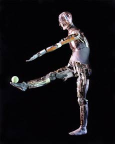
     There was a time at the dawn of computer science, when much hope was put in the area of Artificial Intelligence. There, people attempted to devise "intelligent" algorithms based on formal logic and proofs. The promise was that in a number of years the methods of formal logic would develop to such heights, that would allow computer algorithms to attain "human" level of intelligence. That is, they would be able to walk like humans, talk like humans and do a lot of other cool things that we humans do. Half a century has passed and this still didn't happen. Computer science has seen enormous progress, but we have not found an algorithm based on formal logic that could imitate intuitive human actions. I believe that we never shall, because devising an algorithm based on formal logic actually means understanding and explaining an action in terms of a fixed number of axioms.

    Firstly, it is unreasonable to expect that we can precisely explain much of the real world, because, strictly speaking, there exist mathematical statements that can't in principle be explained. Secondly, and most importantly, this expectation contradicts the assumption that most "truly human" actions are intuitive, i.e. we are simply incapable of understanding them.

    Now what follows is a strange conclusion. There is no doubt that sooner or later computers will get really good at performing "truly human" actions, the trend is clear already. But, contradictory to our expectations, the fact that we shall create a machine that acts like a human will not really bring us closer to understanding how "a human" really "works". In other words, we shall never create Artificial Intelligence. What we are creating now, whether we want it or not, is Artificial Intuition.

    Tags: , , , ,

  • Posted by Konstantin 13.11.2008 1 Comment
    Lightbulb

    It is good to attend lectures from time to time, even if these are on the topics that you "already know". Because, once in a while, you get to find out something new about things that are so "simple" and "familiar", that you thought there was nothing new you could possibly discover about them. So, today I've had an accidental revelation regarding a simple yet amusing property of the maximum likelihood estimation method. I think I should have been told that years ago, right on the first statistics course.

    Maximum Likelihood

    Maximum likelihood estimation is one of the simplest and most popular methods for fitting mathematical models to given data. It is most easily illustrated by an example. Suppose you are given a list of numbers (x_1, x_2, \dots, x_n), which, you believe, are all instances of a normally distributed random variable with mean \mu and variance \sigma^2. The problem is that the value of \mu is unknown to you and you would like to estimate it from the data. How do you do it? The maximum likelihood method suggests you to search for a value of \mu, for which the probability (or probability density) of obtaining exactly this set of numbers would be maximal. That is:

    \hat\mu = \mathrm{argmax}_{\mu} P[x_1, x_2, \dots, x_n\,|\,\mu]

    In most cases this turns out to be quite a reasonable suggestion, which leads to good estimates (although, there are some rare exceptions). Here, for example, it turns out that to estimate the mean you should simply compute the average of the given numbers:

    \hat\mu = \frac{1}{n}\sum_i x_i

    This is more-or-less all what a typical textbook has to say about maximal likelihood, but there's more to it.

    Counting Lightbulbs

    Consider the following example. Suppose you are willing to measure the average lifetime of a common lightbulb (that is, the amount of time it will glow until burning out). For that you buy 1000 lightbulbs in a general store, switch all of them on and wait for a year, keeping track of the timepoints at which the  individual lightbulbs burn out. Suppose the year has passed and you managed to record the lifetime of just 50 "dead" lightbulbs (the remaining 950 keep on glowing even after the whole year of uninterrupted work). What do you do now? Do you wait for other lightbulbs to burn out? But this can take ages! Do you just discard the 950 lightbulbs and only consider the 50 for which you have "available data"? This is also not good, because, clearly, the knowledge that 95% of lightbulbs live longer than a year is important. Indeed, from this fact alone you could infer that the average lifetime must be between 18 and 21 years with 95% confidence (an interested reader is invited to verify this claim). So what do you do?

    Assume that the lifetime of a lightbulb can be modeled using exponential distribution with mean \lambda (this is a natural assumption because exponential distribution is well-suited for describing the lifetime of electric equipment). Then the probability (probability density, in fact) that lightbulb i burns out after t_i years can be expressed as:

    P[X=t_i\,|\,\lambda] = \frac{1}{\lambda}e^{-\frac{t_i}{\lambda}}.

    Naturally, the likelihood of lightbulbs 1,2,3,...,50 burning out after t_1,t_2,\dots,t_{50} years correspondingly, is just the product of the corresponding expressions:

    \prod_{i=1}^{50}\frac{1}{\lambda}e^{-\frac{t_i}{\lambda}}.

    Now what about the lightbulbs that are still alive? The likelihood that a lightbulb will glow longer than a year can be easily expressed as:

    P[X > 1\,|\,\lambda] = e^{-\frac{1}{\lambda}}.

    Therefore, the total likelihood of having 50 lightbulbs burn out at time moments t_1,t_2,\dots,t_{50} and 950 lightbulbs keep working longer than a year is the following product:

    P[X_1 = t_1, X_2 = t_2, \dots, X_{50} = t_{50}, X_{51} > 1, \dots, X_{1000} > 1|\,\lambda] =
    = \left(\prod_{i=1}^{50}P[X_i = t_i\,|\,\lambda]\right) \cdot \left(P[X > 1 \,|\,\lambda]\right)^{950} =
    = \left(\prod_{i=1}^{50}\frac{1}{\lambda}e^{-\frac{t_i}{\lambda}}\right)\cdot e^{-\frac{950}{\lambda}}.

    Finding the estimate of \lambda that maximizes this expression is now a simple technical detail of minor importance. What is important is the ease with which we managed to operate the "uncertain measurements" for the 950 lightbulbs.

    Final Remarks

    Note that the idea can be extended to nearly arbitrary kinds of uncertainty. For example, if, for some lightbulb we knew that its lifetime was a number between a and b, we would include this piece of knowledge by using the term P[a < X < b] in the likelihood function. This inherent flexibility of the maximum likelihood method looks like a feature quite useful for the analysis of noisy data.

    Surprisingly, however, it does not seem to be applied much in practice. The reason for that could lie in the fact that many nontrivial constraints on the data will make the likelihood function highly nonconvex and hard to optimize. Consider, for example, the probability density

    P[X = x_1 \vee X = x_2 \vee X = x_3 \,|\,\lambda] = P[x_1\,|\,\lambda] + P[x_2\,|\,\lambda] + P[x_3\,|\,\lambda]

    for a normally distributed variable X. Depending on the choice of x_1, x_2, and x_3, the likelihood function will have either three different peaks at \lambda = x_1, x_2, x_3, two peaks or just one. Thus, finding an exact optimum is much harder than in the typical textbook case. But on the other hand, there are various cases where the likelihood function is nicely convex (consider the interval constraint mentioned above) and besides there are numerous less efficient algorithms around anyway. So maybe the trick is not used much, simply because it's not in the textbook?

    Tags: , ,