• Posted by Konstantin 19.06.2010 1 Comment

    The other day I was working on a Python program, which internally used a data structure for holding a set of rules. Each rule specified how some object was created from some other objects through certain procedures. The corresponding set of rules could be represented as a bunch of assignment expressions:

    # Description of the relations between objects
    some_item[1].sub_item = some_proc(other_item[2], "Text", 42)
    some_item[2].sub_item = other_proc(some_item[1], "Text", 1337)
    # ... etc

    I would manually describe the required structure using code like the following (in fact, it was slightly more complicated than that, but I hope you get the point).

    struct = Structure()
    struct.add_relation(['some_item', '[1]', '.sub_item'], 
                     ['some_proc', ['other_item', '[2]'], '"Text"', '42'])
    struct.add_relation(['some_item', '[2]', '.sub_item'],
                     ['other_proc', ['some_item', '[1]'], '"Text"', '1337'])
    now_do_something_with(struct)

    After having specified the required rules I would process them and thus solve my task, the details of which are not important here. What is important, is that all those struct.add_relation lines looked messy, long and ugly, and begged for a more concise syntax.

    One obvious choice would be to write the expressions down as strings and parse them within add_relation using ast.parse:

    struct = Structure()
    struct.add_relation(
      'some_item[1].sub_item = some_proc(other_item[2], "Text", 42)')
    struct.add_relation(
      'some_item[2].sub_item = other_proc(some_item[1], "Text", 1337)')
    now_do_something_with(struct)

    Multiple variations on this idea are possible (for example, the whole description could go in a separate configuration file), but in any case this is not a very "easy" solution.

    What I am going to show you here is that appropriate use of Python's dynamic features makes it possible to have the structure defined using Python code, side-by-side with normal Python code, in the following manner:

    @structure_definition
    def struct():
       some_item[1].sub_item = some_proc(other_item[2], "Text", 42)
       some_item[2].sub_item = other_proc(some_item[1], "Text", 1337)
    
    now_do_something_with(struct)

    This post aims to explain the mechanics behind such a solution.

    Part I: __getattr__ and __setattr__

    The first step is fairly easy. As you should know, Python is fairly flexible in that it allows you to redefine any operator, including attribute access, function invocation and assignments. We can therefore create a class StructureCreator, which does redefine all those operators as needed, and then use it in the following manner:

    s = StructureCreator()
    s.some_item[1].sub_item = s.some_proc(s.other_item[2], "Text", 42)
    s.some_item[2].sub_item = s.other_proc(s.some_item[1], "Text", 1337)

    To see what we need to do to make it work, let us explicitly write out what happens here on line 2. This line is equivalent to the following expression:

    s.__getattr__('some_item')
     .__getitem__(1)
     .__setattr__('sub_item', 
       s.__getattr__('some_proc')
        .__call__(s.__getattr__('other_item').__getitem__(2), "Text", 42)
     )

    This invocation structure neatly corresponds to the parse tree of the original expression and our StructureCreator class should therefore simply collect the information from the invocations, recursively building data structures describing the left- and right-hand sides of the expression. Finally, at the time the assignment operator __setattr__ is invoked, the collected information about the assignment can be saved appropriately. Here is an abridged conceptual example:

    class StructureBuilder:
      def __init__(self, expr=''):
        self.__dict__['__expr__'] = expr
    
      def __str__(self):
        return self.__expr__
      __repr__ = __str__
      
      def __getattr__(self, attrname):
        newname = self.__expr__ + '.' + attrname
        return StructureBuilder(newname)
    
      def __setattr__(self, attrname, val):
        newname = self.__expr__ + '.' + attrname
        print 'Saving: %s = %s' % (newname, str(val))   
    
    s = StructureBuilder()
    s.x = s.y

    It remains to implement __getitem__, __setitem__ and __call__ in a similar manner, and voila, you are all covered in syntax sugar.

    The fact that you will have to prefix all your "custom" expressions with this annoying s. might still bug your aesthetical feelings. If so, follow me to the next step.

    Part II: Hiding the Builder

    In the previous part we figured out how, by using __getattr__ and __setattr__ we can make Python interpret assignments our way. In order for it to work, however, we need to explicitly refer to an object which implements those methods, and write lines like

    s.x = s.y

    Can we somehow "hide" this object and have something analogous to automatic __getattr__ for global scope? Yes we can: Python conveniently provides us with a construction:

    exec [code] in [environment]

    which would execute our code, using the provided dictionary to resolve variables.

    Let us try it. We modify our StructureBuilder to inherit from dict and add the methods __getitem__ and __setitem__ which will happily resolve and assign to arbitrary variable names:

    class StructureBuilder(dict):
      def __init__(self, expr=''):
        self.__dict__['__expr__'] = expr
    
      def __str__(self):
        return self.__expr__
      __repr__ = __str__
      
      def __getattr__(self, attrname):
        newname = self.__expr__ + '.' + attrname
        return StructureBuilder(newname)
    
      def __setattr__(self, attrname, val):
        newname = self.__expr__ + '.' + attrname
        print 'Saving: %s = %s' % (newname, str(val))   
    
      def __getitem__(self, itemname):
        newname = self.__expr__ + '.' + str(itemname)
        return StructureBuilder(newname)
    
      def __setitem__(self, itemname, val):
        newname = self.__expr__ + '.' + str(itemname)
        print 'Saving: %s = %s' % (newname, str(val))
    

    Does it work?

    s = StructureBuilder()
    exec 'x[1].y = z' in s

    It does, but now we are providing Python code in a string, which is not at all sexy. Let us try the following instead:

    def definition():
      x[1].y = z
    
    exec definition.func_code in s

    Bummer. NameError: global name 'z' is not defined.. But why? Isn't that exactly the same as the previous attempt with a string?

    Part III: Lexical Scoping

    There is a difference in how Python compiles code in a string and in a function. To see that, let us take a look at what's inside the compiled snippets for a string

    s = 'x = y'

    and a function

    def f():
      x = y

    To do that let us use Python's bytecode disassembler module dis:

    import dis
    # First snippet (code in a string)
    dis.dis(compile(s, '', 'exec'))
    # Second snippet (code in a function)
    dis.dis(f.func_code)

    Here is the output for two snippets side by side:

    Snippet1 (String)                Snippet2 (Function)
    -------------------------------------------------------
    0 LOAD_NAME      0 (y)           0 LOAD_GLOBAL    0 (y)
    3 STORE_NAME     1 (x)           3 STORE_FAST     0 (x)
    6 LOAD_CONST     0 (None)        6 LOAD_CONST     0 (None)
    9 RETURN_VALUE                   9 RETURN_VALUE 

    Now we see it - the snippet from the string uses the LOAD_NAME and SAVE_NAME commands to access the variables, which neatly proxy the requests to our dictionary, as we want them to.

    The snippet from the function behaves in a different way. Firstly, the variable x is accessed using STORE_FAST, which is a command used for local variables. This command would not use the provided dictionary because the variable x has been determined as local to the function's scope and assigned its own memory location within the function's frame at compilation. Secondly, the variable y is accessed via LOAD_GLOBAL which, in Python's terms, refers to a variable from a surrounding lexical scope, not the dynamic scope we are trying to enforce. In short, this command also does not care about the dictionary that we provided.

    Does it mean that it is impossible to overcome the scoping rules that Python uses when compiling a function? Of course not - all we need is to modify the bytecode, replacing each LOAD_FAST, STORE_FAST, LOAD_GLOBAL and STORE_GLOBAL with LOAD_NAME and STORE_NAME.

    Part IV: Bytecode

    The required modification is well documented here, but let me give you a brief overview.
    The bytecode for a Python function f is stored in its field f.func_code.co_code. It is a sequence of bytes, which is easy to parse into opcodes. Every opcode is one byte long. Opcodes with a byte-value greater or equal than opcode.HAVE_ARGUMENT are followed by a two-byte argument. This does not seem to be well documented, but is easily read out from the code of the dis.dis function, which comes with Python. For completeness' sake, here's how a simple bytecode parser might look like:

    def bytecode(code_obj):
    	import opcode
    	code = code_obj.co_code
    	n = len(code)
    	i = 0
    	while i < n:
    		op = ord(code[i])
    		i += 1
    		oparg = None
    		if op >= opcode.HAVE_ARGUMENT:
    			oparg = ord(code[i]) + ord(code[i+1])*256
    			i += 2
    		yield (op, oparg)
    

    We now need to take the code object of our function, replace the ***_FAST and ***_GLOBAL commands with ***_NAME and create a new code object. Leaving out some details, this goes as follows:

    def as_anonymous_block(func):
      new_bytecode = []
      for (op, arg) in bytecode(func.func_code):
        if (op in [STORE_FAST, LOAD_FAST, STORE_GLOBAL, LOAD_GLOBAL]):
          new_op = LOAD_NAME or STORE_NAME, correspondingly
          new_arg = for ***_FAST we need to modify this value
          new_bytecode.append(new_op, new_arg)
        else:
          new_bytecode.append(op, arg)
      return types.CodeType( ... options, flags ... , new_bytecode)
    

    Once we perform this modification on our function object, we can use exec ... in ... to have our StructureBuilder take control of the assignments within the function:

    def definition():
      x[1].y = z
     
    exec as_anonymous_block(definition) in s
    

    Part V: Putting It All Together

    As I promised in the beginning of this post, it is possible to encapsulate the whole thing into a function annotation @structure_definition and use it as follows:

    @structure_definition
    def struct():
       some_item[1].sub_item = some_proc(other_item[2], "Text", 42)
       some_item[2].sub_item = other_proc(some_item[1], "Text", 1337)
    
    now_do_something_with(struct)

    The last step is therefore creating the @structure_definition annotation, which is rather straightforward. For a given function it processes it using as_anonymous_block, creates a new StructureBuilder object, executes the function's code in the StructureBuilder, and returns the result:

    def structure_definition(f):
      blk = as_anonymous_block(f)
      result = StructureBuilder()
      exec blk in result
      return result
    

    For further details refer to (a slightly more elaborate) example code here.

    To conclude, I should note that in my case I still ended up using the solution from Step I (i.e. the one where "dynamic" variables are prefixed with s.), because it allows to use loop variables and other constructs alongside my structure definitions much more naturally than the second method. Nonetheless, I hope you enjoyed the presented exploration as much as I did.


    Tags: , , , ,

  • Posted by Konstantin 12.02.2010 4 Comments

    Statistics is mainly about using the observed data to make conclusions about the "real state of affairs", underlying that data. A classical and most widely spread technique for making these conclusions is based on significance testing. In simple terms, the idea of significance testing is to ask the question: "if the real state of affairs were X, how probable would it be for us to obtain the data D we are currently observing?". If the answer is "rather unprobable" (e.g. p < 0.05), the common decision is to reject the proposition X in favor of the alternative "not X". Otherwise the researcher claims to "see no reason to reject X".

    The logic behind that reasoning seems quite solid from the first glance, yet it is well known to be faulty. Naturally, the fact that the likelihood of the data P(D | X) is low need not imply that the underlying hypothesis is wrong - it might very well be the case that the data by itself is already rare enough to make this value low. The only correct way of making sound judgments is to consider the a-posteriori probability of the hypothesis P(X | D) instead. However, the latter can be quite inconvenient to compute. Besides, the wild popularity of significance tests and p-values seems to indicate that the issue is not at all that serious. Really, P(X | D) looks so similar to P(D | X), who cares?

    Book cover

    The book "What If There Were No Significance Tests?", which I stumbled upon recently while browsing a stray library shelf, makes it clear that this issue is not a joke. It is a collection of chapters written by renowned statisticians (most of which some-why work in the field of psychology), that quite convincingly condemns the widespread overuse of p-values and the related significance-based hypothesis testing in favor of other approaches. The main point is nailed quite precisely in the very first essay by Jacob Cohen, which I strongly advise you to read right now in order to get rid of any illusions you might still have regarding significance testing. And when you're done with that, you can continue reading this post.

    In the following I shall provide my personal summary of the marvelous "Member of Congress" example from J.Cohen's essay. So far it is the best illustration I know of, about why exactly it is dangerous to use significance tests blindly.

    Improbable does not mean impossible

    Consider the following situation. We have observed a person which we know to be a Member of the US Congress. We are interested in testing the hypothesis, that this person is an American citizen. To apply the significance testing methodology, we proceed by estimating the p-value:

    P(Congressman | American) ~ 535/300 000 000.

    This is clearly below the popular 0.05 threshold. As a result, we are forced to reject the null-hypothesis and conclude that the person is not an American citizen. Bummer.

    What is the problem here? Well, one thing is worth noting - while the probability for an American to be a congressman is low, it is even lower (precisely, zero), for a non-American. So maybe we would have been better off if we expanded the procedure above to the following "maximum-likelihood"-style reasoning:

    Considering that the likelihood P(Congressman | American) is greater than the likelihood P(Congressman | non-American), we must conclude that the person in front of us is an American rather than not.

    Did we just solve the problem? Is it enough to consider "p-values both ways" to clear things up? No!

    Maximum likelihood does not work

    Let us now consider a reversed situation. We are faced with a person, which, we know, is an American. We are interested in the hypothesis that he is a congressman. Compute the two likelihoods:

    P(American | Congressman) = 1

    P(American | not Congressman) ~ 300 000 000 / 6 700 000 000

    Observing that the first likelihood is greater than the second we are forced to conclude that the person in front of us is indeed a congressman. Bummer, again!

    Only by multiplying the likelihood with the marginal probability P(Congressman) could we have obtained the correct decision. Which is, to say, we must have been estimating the probabilities the other way around from the start.

    To summarize, be wary of these pitfalls. I would not agree with the strong negative opinion of the authors of the book, though. After all, a lot of stuff is quite fruitfully done nowadays using p-values only. However, each time you use them, do it sensibly and keep in mind the following two aspects:

    1. If your p-value is low, can this be solely due to low marginal probability of the data? What is the "reversed" p-value? What is the power of your test?
    2. If you suspect that your hypotheses might be subject to a highly non-uniform prior probabilities, do not use bare p-values. You must consider the prior!

    Tags: , ,

  • Posted by Konstantin 21.11.2009 1 Comment

    In the recent weeks I had to give a few introductory lectures on supervised machine learning within Jaak's data mining course. I also provided the students some home assignments, and there it was especially tricky to find a simple, fun and discussable exercise, which might help to form some intuition regarding the inherent difficulties of learning from data such as overfitting, multiple testing, and the like. The following is what I came up with and I find it a rather successful creation. It is remarkable that of the 80 students participating in the course only 4 or so came up with the correct answer 🙂

    The Riddle

    After the lecture on supervised machine learning at the University of Mordor, the teacher, Sauron, gave the students a dataset of the following form:

                1) ABACDAFXYZ    -> good
                2) CEGXEAELWMN   -> good
                3) NUWAB         -> bad
                        ...
               20) QRELAZMNPCXA  -> good

    The inputs were seemingly arbitrary strings of latin characters: these were the terrible spells known only to Sauron and chosen by Sauron at random from his Great Book of Terrible Spells. The output was a binary variable, classifying each spell as good or bad. There were 20 observations in total in the dataset.

    The students were given a task: on the basis of this data, come up with a generic spell classifier. Sauron promised to test their result on the next lecture as follows: he will pick another random terrible spell from the book and require each student to make a prediction. The student whose prediction is wrong will have to jump down from the tower as a punishment.

    The first student, Aghargh, who happened to be slacking on the lecture, couldn't come up with any smart ways to solve the task, so he ended up just counting the proportion of "good" and "bad" spells in the dataset. Having observed that 16 of the 20 spells were "good", he decided to predict "good" when asked.

    The second student, Bughrorc, chose a smarter way. Firstly, he converted each string into a vector of binary attributes — one attribute for each letter, having value "1" if that letter was present in the corresponding spell and "0" otherwise. He then split the data randomly into a training set (15 instances) and a test set (5 instances), and attempted training various classifiers using the MordorMiner software. After some experimenting he finally found five classifiers that could predict all of the training examples correctly. One of these also predicted all of the testing examples correctly. He decided to use this classifier on the forthcoming test.

    On the day of testing, Sauron asked the students to classify the spell YOZAZA. Aghargh, as he decided, provided the answer "good". Bughrorc's classifier analyzed the string and claimed that the answer should be "bad"

    Which of the students, do you think, might have a better chance of not jumping from the tower? Why? Can you quantify your answer?

    Tags: , , ,

  • Posted by Konstantin 23.10.2009 No Comments

    The Alt+Tab key combination is perhaps one of the most well-known keyboard shortcuts in Windows, with the only competitors for the throne being Ctrl+C and Ctrl+V. And no matter, whether you are used to alt-tabbing for working purposes or simply as a means of efficient undercover procrastination, unless you are a complete novice you probably have this skill at the level of basic instincts.

    Unfortunately, there are cases where the instinct becomes inconvenient. Namely, whenever you use an application that displays multiple documents in separate tabs (like Firefox or Notepad++) or in separate child windows (like R), you are expected to use Ctrl+Tab rather than Alt+Tab to switch among documents. However, most of the time switching among documents is subjectively perceived as nothing essentially different than switching among programs, hence the fact that Alt+Tab won't work normally for that case is highly unintuitive. The typical case with me is that I would accidentally use Alt+Tab attempting to switch between the editor and console in R and unexpectedly find a completely different window in front of me, which is quite annoying.

    Although I am pretty sure I am not the only one to experience this kind of frustration, it is surprising that there does not seem to be any easily available solution to this trivial issue known to google. Thus, considering that the whole problem can be solved to a fair extent by simply translating Alt keypresses into Ctrl in a smart way, I've made a smallish program that does exactly that.

    I'm quite happy with the result and can't help sharing it with you.

    Download: Binary, Source.

    Tags: , , ,

  • Posted by Konstantin 11.10.2009 2 Comments

    I've recently stumbled upon a simple observation, which does not seem to be common knowledge and yet looks quite enlightening. Namely: polynomials provide an excellent way of modeling data in an order-agnostic manner.

    The situations when you need to represent data in an order-agnostic way are actually fairly common.  Suppose that you are given a traditional sample x_1, x_2, \dots, x_n and are faced with a task of devising a generic function of the sample, which could only depend on the values in the sample, but not on the ordering of these values. Alternatively, you might need to prove that a given statistic is constant with respect to all permutations of the sample. Finally, you might simply wish to have a convenient mapping for your feature vectors that would lose the ordering information, but nothing else.

    The most common way of addressing this problem is sorting the sample and working with the order statistics x_{(1)}, x_{(2)}, \dots, x_{(n)} instead of the original values. This is not always convenient. Firstly, the mapping of the original sample to the corresponding vector of order statistics (i.e. the sorting operation) is quite complicated to express mathematically. Secondly, the condition that the vector of order statistics is always sorted is not very pleasant to work with. A much better idea is to represent your data as a polynomial of the form

        \[p_x(z) = (z+x_1)(z+x_2)\dots(z+x_n)\,.\]

    This will immediately provide you with a marvellous tool: two polynomials p_x and p_y are equal if and only if their roots are equal, which means, in our case, that the samples x_1,\dots,x_n and y_1,\dots,y_n are equal up to a reordering.

    Now in order to actually represent the polynomial we can either directly compute its coefficients

        \[p_x(z) = z^n + a_1z^{n-1} + \dots + a_n\,,\]

    or calculate its values at any n different points (e.g. at 0,1,\dots,n-1) - in any case we end up with the same amount of data as we had originally (i.e. n values), but the new representation is order-agnostic and has, arguably, much nicer properties than the order statistics vector.

    It is not without its own problems, of course. Firstly, it requires at least \Omega(n^2) time to compute. Secondly, not every polynomial will have n real-valued roots. And thirdly, the interpretation of the new "feature vector" is not necessarily intuitive or meaningful. Yet nonetheless, it's a trick to consider.
    Tags: , , , ,

  • Posted by Konstantin 11.08.2009 7 Comments

    Inspired by Swen

    Tags: , , ,

  • Posted by Konstantin 25.06.2009 No Comments

    Every Spring thousands of aspiring undergraduates spend numerous diligent hours working on their final theses, suffering the stress of the deadlines and the tempting pressure of the nice weather. Once they are done writing, they defend their work in public. In the end, they are graded by their supervisors, opponents and an academic committee. The grading rules might vary among universities and faculties, but their essence can be abstracted as follows: the supervisor provides a mark representing his opinion, the opponent provides a mark representing his opinion, and the final grade is obtained by taking the average of the two.

    However, this process is not necessarily as simple as it looks like from the first glance. Although both the supervisor and the opponent are supposed to announce "the mark, representing their opinion", they are knowledgeable of the final grading scheme and might in fact, perhaps unconsciously, play a somewhat different game. Indeed, if the supervisor believes the student's work is worth a 4, he is in fact interested that final grade would be 4, no more and no less. The same holds for the opponent. Now let us assume that the difference between the proposed mark and the final mark measures the "penalty" for both the supervisor and the opponent. We could then regard the whole grading process as the following game.

    • The supervisor has his opinion about the proper mark s \in \{1,2,3,4,5\}. Similarly, the opponent has his opinion about the proper mark o \in \{1,2,3,4,5\}.

    • The supervisor announces the mark s' \in \{1,2,3,4,5\}, the opponent announces the mark o' \in \{1,2,3,4,5\}. The final grade f is computed as the average (s'+o')/2.
    • The supervisor receives penalty \mathrm{abs}(s-f) and the opponent receives penalty \mathrm{abs}(o-f).
    • Naturally, both parties are interested in minimizing the penalty.

    Now, assuming that both the supervisor and the opponent are indeed playing the above game, how would they act? Of course, this depends on their "true" opinions s and o, and whether they are knowledgeable of each other's opinion or not. For simplicity, let us first consider the case where s = o = 4 and both parties know it. In this case, we can represent the game in the traditional matrix form:

    s' o'
    1 2 3 4 5
    1 3 2.5 2 1.5 1
    2 2.5 2 1.5 1 0.5
    3 2 1.5 1 0.5 0
    4 1.5 1 0.5 0 0.5
    5 1 0.5 0 0.5 1
    Penalty for both supervisor and opponent for various choices of s' and o'

    There are three optimal solutions here — (s'=3,o'=5), (s'=4,o'=4) and (s'=3,o'=5), with the logical (4,4) choice being the "safest" for both parties in terms of the maximal possible penalty in case the opposing party presumed a different optimal solution.

    Now what if s and o are different. For example, s = 4 and o = 3. In this case, the payoffs of the supervisor and the opponent are not equal any more:

    s' o'
    1 2 3 4 5
    1 3 | 2 2.5 | 1.5 2 | 1 1.5 | 0.5 1 | 0
    2 2.5 | 1.5 2 | 1 1.5 | 0.5 1 | 0 0.5 | 0.5
    3 2 | 1 1.5 | 0.5 1 | 0 0.5 | 0.5 0 | 1
    4 1.5 | 0.5 1 | 0 0.5 | 0.5 0 | 1 0.5 | 1.5
    5 1 | 0 0.5 | 0.5 0 | 1 0.5 | 1.5 1 | 2
    Penalties for supervisor and opponent (separated by | ) for various choices of s' and o'

    There are two Nash equilibrium solutions to this game and it is funny to see that none of them is the seemingly logical (4,3) choice. Instead, they are (5,1) and (1,5), the former being somewhat preferable to the supervisor. That means, the equilibrium strategy dictates the supervisor to suggest the mark 5 (which exceeds his opinion), to which the opponent should respond with a drastically low evaluation of 1. Looks like a rather typical thesis defence scenario, doesn't it? 🙂

    Finally, when the true s and o are not known by the opponent and the supervisor correspondingly, the analysis becomes more complicated, because the players now have to assume something about the opponent. But the conclusion stays the same — whenever the supervisor has the slightest doubt that the opponent might be willing to suggest a lower mark, he will have to pick the overestimation strategy. And the opponent will then naturally tend to drastically underestimate.

    By this weird post I actually wanted to express sincere congratulations to those who have succesfully defended this year, in particular my diligent bachelor students Anastasia, Karl and Riivo.

    Tags: ,

  • Posted by Konstantin 30.03.2009 No Comments

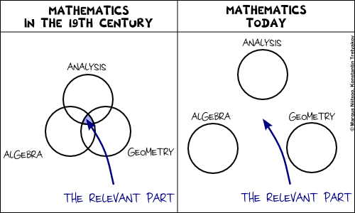
    A cute joke by Margus from the recent EWSCS09 Crapcon session.

    Tags: , , , ,

  • Posted by Konstantin 26.03.2009 No Comments

    Symbols and Reality

    Mathematics is a language. An abstract set of generic symbols for describing concepts, objects and systems. Take, for example, the symbol "5", "five". What is it? Is it a real-world object? No. It is just a symbol. You are free to attach to it any interpretation that you deem appropriate. Of course, most of the times you would use the common interpretation of "5" as a natural number, denoting, well, "five of something". Literally meaning that you can count something as "this, this, this, this and this".

    Take a moment to reflect on the degree of generality of this simple concept, "five". It can be applied to practically anything. Five apples, five centimeters, five centuries are notions as different from each other as you could imagine, and yet all of them relate to the concept "five". On the other hand, it is not too generic to be useless: "five" is radically different from "six", "seven", and an infinity of other numbers. This kind of magical balance between generality and specificity is common to mathematics. This is what makes mathematics both widely applicable and yet still incredibly useful.

    Besides just giving us symbols like 5 or 6, mathematics provides an endless variety of ways for expressing "rules", "operations", "statements", "derivations", "computations" and the like, such as 5+5=10, or \forall x:\, x^2 - 10x \gt -5^2, etc. Once again, all of these rules, operations and statements need not necessarily bear any relation with reality. After all, they all are just a cunning play with symbols. And yet, quite often they do describe reality incredibly well. I know that 512 apples and 512 apples will make 1024 apples together. How do I know it? Certainly not because I checked it on real apples! I just believe that the real-world operation of "adding apples" can be satisfactory modeled using the formal symbolic framework of natural numbers and the operation of addition on them. Why do I believe it? This is a tricky philosophical question that we shall leave aside for now. But remember that any application of mathematics to the real world is always based on a belief that the chosen model describes the world well.

    The Nature of Uncertainty

    There are often cases where we would like to use mathematics to model "uncertainty". Now remember that from the point of view of pure math there are no such things as inherent "certainty" and "uncertainty". Mathematics will always operate on symbols and use precise, uniquely reproducible transformation rules between these symbols. Yet there are often cases when we, in our interpretations of these symbols, would like refer to certain entities as "uncertain". The reasons can be various:

    1. Sometimes, we would like to use a single generalized concept to summarize multiple objects.
      - What is the height of a human?

      There is no single clear answer and yet it is possible to provide one using an uncertainty model such as a probability distribution.
    2. Sometimes, we want to reason about some single numeric value which, even if it were well-defined, we just could not compute exactly.
      - What is the AVERAGE height of a human?

      In theory, it is a number you could measure by lining up all the people in the world and computing their average, but it is certainly an infeasible project.
    3. Sometimes, the notion we would like to reason about is inherently not well-defined.
      - What is MY height, after all?

      The answer depends on a number of factors such as time, measuring equipment, my precise posture, etc. Instead of taking all of these into consideration, we prefer to exploit an uncertainty model.
    4. Sometimes we just need a single concept to encapsulate a state of knowledge more sophisticated than pure numeric equality. For example, to express the fact like "my height IS GREATER THAN 150cm" without using the "greater than" operation.

    There are also other situations, which are difficult to classify, but in all cases the idea is the same — for one reason or another we "don't know" (or "don't specify") the exact single quantity we want to reason about, an yet we still "know something" about it. In fact, amusingly, the amount of information that we use to represent an "uncertain" quantity is often much greater than the amount of information we would need to represent a "certain" one. For example, there are much more probability distributions than there are real numbers. Therefore, picking one probability distribution to represent our knowledge of a number is, in principle, a more informative step than picking a single real number. And yet, we call the former case "uncertainty" and the latter one "certainty". Because that's how we choose to name and interpret things, that's how we believe these concepts relate to reality.

    Models of Uncertainty

    The adjective "uncertain" is something you could, in theory, apply generically to any type of data. In a computer scientist's terms, it makes perfect sense to talk about datatypes "uncertain int", "uncertain real", "uncertain boolean", "uncertain string", "uncertain graph", "uncertain map" and maybe even "uncertain uncertain real" and the like. Let's limit ourselves here to the consideration of uncertain numbers only, as these are the most commonly used and well-studied types of uncertainty. So how do you model (or, say, "implement") "uncertain real"? Here is a short list of the most popular options:

    1. Approximate numbers.Although you might not consider it as a smart approach, this is probably the most common choice in practice — using a usual number to represent an uncertain one. In this case the uncertainty is purely interpretative: instead of stating x = 5 you would, perhaps, write x \approx 5, denoting your state of ignorance. Quite often you would not even care to use the approximate equality sign, presuming it is clear from the context that you are not supposed to provide an ideally exact measurement: — What is your height? — It is 180cm. This works quite well in simple real-life situations, such as buying a kilogram of apples or discussing the horsepowers in a friend's motorbike, but is also applicable to some more technical cases, such as computing the distance to the nearest star.The advantage of such implied uncertainty is that you do not really need to deal with it. All of your familiar arithmetic operations come for free, together with their well established interpretations and the nice properties, theories and theorems. The disadvantage is that once your data is approximate, all of these theories and theorems become approximate too. So, although it could often be acceptable to claim x \approx 5, y \approx 10 \Rightarrow x + y \approx 15, you would have problems explaining more complicated steps, such as "x \approx 5 \Rightarrow f(x) \approx f(5) for a continuous f".But what to do if you need to perform such steps? Consider intervals instead!

    2. Intervals.The second most popular method of representing an uncertain real number is to provide an interval where it falls into. It is ubiquitous in engineering disciplines. Most often an interval is expressed either as x\pm\Delta x or by following the significant figures convention (e.g. writing 180.00 to denote 180±0.01). It is an improvement over the previous approach, because now you have a way to quantify the effect of function application on uncertainty. For example, a commonly used rule would be

      f(x\pm\Delta x) \approx f(x)\pm\left(\frac{\partial f(x)}{\partial x} \Delta x\right),

      where f is a differentiable function.

    3. Sets.An approach slightly more general than the "interval" technique would be to provide a set of values, to which the value of interest could belong to. So, instead of stating x = 5 you could write, for example, x \in \{4,5,7\}.This allows for more mathematical rigour. For example: x \in \{4,5,7\} \Rightarrow f(x) \in \{f(4), f(5), f(7)\}. Moreover, besides the standard algebraic operations, the set representation allows to update the knowledge about an uncertain value easily using set unions and intersections:


      x \in A, x \in B \Rightarrow x \in A\cap B.

      However, sets are "heavy" object to work with, so you don't see this approach being used too often in practical computations. Some Monte-Carlo simulations would use a set to represent approximate solutions, but they would convert it to a probability distribution as soon as possible. This leads us to the next item on the list.

    4. Probability distributions.If the previous methods were either too crude, too ad-hoc or too heavy, then probability theory was designed to provide flexible balance and help overcome most of their drawbacks. To represent a number it suggests us to use a probability measure - an additive function that assigns a weight to each set, which could contain the value of interest. The greater the weight of a set - the more probable it is that the value belongs to that set. By convention, the minimum possible weight of a set is 0, which we usually interpret as "the value almost certainly does not belong to that set", and the maximum weight is 1, with a corresponding interpretation "the value almost certainly belongs there". Representing a function defined on sets is complicated, so usually we use a simpler equivalent representation: a cumulative distribution function (CDF) or a probability density function (PDF). The plot of the latter is especially insightful and provides a nice visual cue about the nature of uncertainty being modeled.It is impossible to enumerate all the virtues of using a probability distribution as an uncertainty model. A probability distribution is a flexible structure, capable of accomodating most "common" kinds of uncertainty. There is an authoritative, well-developed theory and a wide range of both practical and theoretical tools available. Besides the standard algebraic operations, you have rules for updating knowledge (such as the Bayes rule) and a range of facilities for decision making (estimation, hypothesis testing, etc). Finally, there are various interpretations available for you to choose from.Of course, there are potential drawbacks, too. On the practical side, it is not always computationally convenient to work with a probability measure. It is a function, after all, and when specified arbitrarily it can either take too much space to represent or too much time to compute. The use of smoothing and approximation techniques can somewhat relieve the problem, but comes at the price of additional assumptions and simplifications. Secondly, a probability distribution is not capable of representing any kind of uncertainty: for example, there is no probability distribution corresponding to the statement "x < 5". Thirdly, the requirement for a probability density to be normalized to sum to 1 is sometimes inconvenient (because you have to normalize) or unintuitive (because it seems to declare that there is a single uncertain value "hidden inside").

      For example, consider the picture on the right and try to provide a concise description of the set of black pixels on it. This will be an uncertain notion because, well, a gray pixel is also somewhat black, isn't it? And although you could provide a probability distribution of "black" on the picture, you would probably intuitively prefer to assign a "truth-value" between 0 and 1 to each pixel, with 1 corresponding to "certainly black" and 0 to "certainly not black". This would, however, violate the "sum-to-one" normalization rule and thus would not be a probability density. What would it be? A fuzzy set.

    5. Fuzzy sets.A fuzzy set is a set whose elements can have a degree of membership between 0 and 1. It is therefore something inbetween a set (because it "feels" like a set) and a probability density (because it is a function, only this time normalized to have a maximum of 1, instead of the integral of 1). A person familiar with probability theory will also easily recognize a straightforward analogy of a fuzzy set to a likelihood function.Fuzzy sets seem to be a natural uncertainty model in various circumstances, such as the "black pixels" example above. They are often conceptually simpler to specify than probability densities, and lack the interpretation controversy surrounding probability theory. On the other hand, the theory of fuzzy sets is not as extensive as that of probabilities. It is rich in operations like max and min, which makes some things computationally difficult. Besides, the lack of a universal interpretation for fuzzy membership values results in a lack of simple unique decision-making facilities. There are just way too many defuzzification rules to choose from.
    6. ... and more.A variety of other approaches is available, the most important ones being Possibility theory, and Dempster-Shafer theory. However, as this text has already grown too long for a blog post, I shall leave the detailed description of these to Wikipedia.

    Summary

    The main message of this exposition is actually quite simple. There are various approaches to modeling uncertainty. They differ in the type of supported operations and, most importantly, in the way we interpret them and map to the real world entities. But nonetheless, these are all still just methods for modeling uncertainty, each with its own advantages and limitations. Moreover, in most situations, as long as you use the math "reasonably", the models are approximately equivalent in terms of the results and decisions you might end up with using them. That is probably the reason why practitioners would rarely consider anything more sophisticated than a probability measure (except, perhaps, when they are feeling adventurous). And that is why it can sometimes be complicated to promote the more "modern" approaches without the awkward looks from the side of the "traditional statistics". After all, these approaches are competing on the same field with The One and Only, Probability Theory.

    Tags: , , , ,

  • Posted by Konstantin 12.03.2009 No Comments

    The yachts parked in the port of Palma de Mallorca might very well outnumber the presumably plentiful palm trees in this city. The photo below depicts just a small piece of the 3 kilometer-long marina, stretched along the Paseo Maritimo coastline.

    Yachts in Palma

    Yachts in Palma de Mallorca

    For the fun of it, let's try counting the yachts on this photo. Even though it is perhaps one of the most useless exercises one might come up with, I find it amusing and not without a relation to a variety of more serious applications. Naturally, no sane computer scientist would attempt to do the counting manually when he can let a computer do this job for him. Therefore, we'll use a chance here to exploit the fantastic Scilab Image Processing toolbox.

    Preprocessing

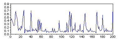
    If we only want to know the number of masts, we don't need the whole image, a single line of the image that crosses all of the masts would suffice. Some pixels of this line will correspond to the sky — a brief examination shows that the RGB colour of these pixels is approximately (0.78, 0.78, 0.78). The remaining pixels will be the masts and the ropes. For each pixel, we can compute how similar this pixel's colour is to the colour of the sky (the simple euclidean distance will do OK), and thus we shall end up with a single vector, the peaks in which will correspond to the masts we need to count.

      // Read image
      img = imread("yachts.jpg");
    
      // Get the proper line
      img_line = img(505,:,:);
    
      // Subtract sky colour
      img_line = sqrt(sum((img_line - 0.78*ones(img_line)).^2, 3));
    The vector to be analyzed

    The vector to be analyzed (its first 200 pixels out of 1600 total)

    Let us now do the counting.

    1. Geometric approach

    A look on the picture above will tell you that a threshold of about 0.2 might be good for discriminating the masts from the background. Once we apply it, there are at least two easy ways to derive the number of masts.

    • Firstly, we could count the number of pixels over the threshold and divide it by four, which seems like roughly the average width of a mast.
         answer = sum(img_line > 0.2)/4

      The result is ~135.

    • Secondly, we could count the number of times the pixel value crosses the 0.2 boundary:
         answer = sum(img_line(2:$) > 0.2  & img_line(1:($-1)) <= 0.2);

      Here the result will be 158.

    2. Spectral approach

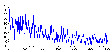
    The discrete Fourier transform of a vector is a natural way for counting repeating peaks in the signal.

      ff = abs(fft(center(img_line)));
      plot(0:300, ff(1:301));


    Masts vector spectrum

    Masts vector spectrum

    The interpretation of the resulting figure should, in theory, be simple. If the photo only contained n uniformly distributed masts, the spectrum would have one clear peak at n. In our case, unfortunately, things do not seem to be as easy. With some wishful thinking one might see major peaks around 50, 150 and 300. Now taking the previous results into consideration let us presume that 150 is the correct peak. Then 50 could correspond to the 50 "larger" masts on the image, and 300, perhaps, to the ropes.

    3. Statistical approach

    The original image is 1600 pixels wide. If the photo contained n masts, distributed uniformly along its width, a randomly chosen 32-pixel region would contain about n/50 masts on average. Therefore, let us select some of these random regions and count the number of masts in them manually. After multiplying the resulting numbers by 50 we should obtain estimates of the total number of masts.

      xbasc();
      rand("seed", 1);
      for i=1:9
        m = floor(rand()*(1600-32))+1;
        subplot(3,3,i);
        imshow(img([474:566], [m:(m+32)],:))
      end

    Here are the estimates I got here: 200, 50, 50, 150, 150, 100, 100, 100, 100. The average comes at 111 with a standard deviation of about 50.

    Summary

    There are serious discrepances among the results produced by various approaches. However, if you attempt to count the masts manually, you will quickly discover that there is indeed an inherent degree of uncertainty in the number of visible masts, with the true number lying somewhere between 100 and 150. Consequently, the considered approaches to mast counting were not too far off, after all.

    Tags: , , ,