Four Years Remaining

This article has been cross-posted to Hackster.

What is the best way to learn (or teach) introductory robotics? What could be the "hello world" project in this field, that would be simple for a beginner to get started with, complex enough to be exciting and qualify as a "robot", and deep enough to allow further creative extensions and experiments? Let us try solving this problem logically, step by step!

First things first: what is a "robot"?

Axiom number one: for anything to feel like a robot, it must have some moving parts. Ideally, it could have the freedom move around, and probably the easiest way to achieve that would be to equip it with two wheels. Could concepts other than a two-wheeler qualify as the simplest robot? Perhaps, but let us proceed with this one as a reasonably justified assumption.

The wheels

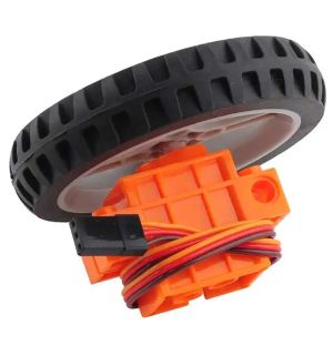
To drive the two upcoming wheels we will need two motors along with all that driver circuitry, ugh! But wait, what about those small continuous rotation servos! They are simple, cheap, and you just need to wire them to a single microcontroller pin. Some of them are even conveniently sold along with with a LEGO-style wheel!

The microcontroller

Rule number two: it is not a real robot, unless it has a programmable brain, like a microcontroller. But which microcontroller is the best for a beginner in year 2024? Some fifteen years ago the answer would certainly have the "Arduino" keyword in it. Nowadays, I'd say, the magic keyword is "CircuitPython". Programming just cannot get any simpler than plugging it into your computer and editing code.py on the newly appeared external drive. No need for "compiling", "flashing" or any of the "install these serial port drivers to fix obscure error messages" user experiences (especially valuable if you need to give a workshop at a school computer class). Moreover, the code to control a wheel looks as straightforward as motor.throttle = 0.5.

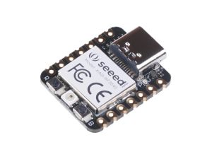
OK, CircuitPython it is, but what specific CircuitPython-compatible microcontroller should we choose? We need something cheap and well-supported by the manufacturer and the community. The Raspberry Pi Pico would be a great match due to its popularity, price and feature set, except it is a bit too bulky (as will become clear below). Check out the Seeedstudio Xiao Series instead. The Xiao RP2040 is built upon the same chip as the Raspberry Pi Pico, is just as cheap, but has a more compact size. Interestingly, as there is a whole series of pin-compatible boards with the same shape, we can later try other models if we do not like this one. Moreover, we are not even locked into a single vendor, as the QT Py series from Adafruit is also sharing the same form factor. How cool is that? (I secretly hope this particular footprint would get more adoption by other manufacturers).

The body

OK, cool. We have our wheels and a microcontroller to steer them. We now need to build the body for our robot and wire things together somehow. What would be the simplest way to achieve that?

Let us start with the wiring, as here we know an obviously correct answer - a breadboard. No simpler manual wiring technology has been invented so far, right? Which breadboard model and shape should we pick? This will depend on how we decide to build the frame for our robot, so let us put this question aside for a moment.

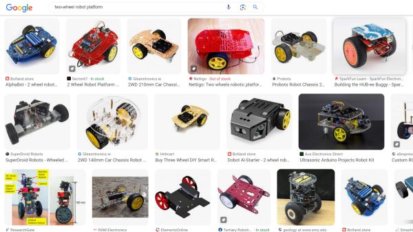
How do we build the frame? The options seem infinite: we can design it in a CAD tool and laser cut it from acrylic sheets, print on a 3D printer, use some profile rails, wooden blocks, LEGO bricks,... just ask Google for some inspiration:

Ugh, this starts to feel too complicated and possibly inaccessible to a normal schoolkid.... But wait, what is it there on the back of our breadboard? Is it sticky tape? Could we just... stick... our motors to it directly and use the breadboard itself as the frame?

If we now try out a few breadboard models, we will quickly discover that the widespread, "mini-sized", 170-pin breadboard has the perfect size to host our two servos:

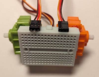
By an extra lucky coincindence, the breadboard even has screw holes in the right places to properly attach the motors! If we now hot glue the servo connectors to the side as shown above, we can wire them comfortably, just as any other components on the breadboard itself. Finally, there is just enough space in the back to pack all the servo wires and stick a 3xAAA battery box, which happens to be enough to power both our servos and the Xiao RP2040:

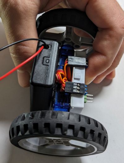
This picture shows the FS90R servos. These work just as well as the GeekServo ones shown in in the picture above.

... and thus, the BreadboardBot is born! Could a breadboard with two motors and a battery stuck to its back qualify as the simplest, lowest-tech ever robot platform? I think it could. Note that the total cost of this whole build, including the microcontroller is under $20 (under $15 if you order at the right discounts from the right places).

But what can it do?

Line following

Rule number 3: it is not a real robot if it is not able to sense the environment and react to it somehow. Hence, we need some sensors, preferably ones that would help us steer the robot (wheels are our only "actuators" so far). What are the simplest steering techniques in introductory robotics? I'd say line following and obstacle avoidance!

Let us do line following first then. Oh, but how do we attach the line tracking sensors, we should have built some complicated frame after all, right? Nope, by a yet another happy design coincidence, we can just plug them right here into our breadboard:

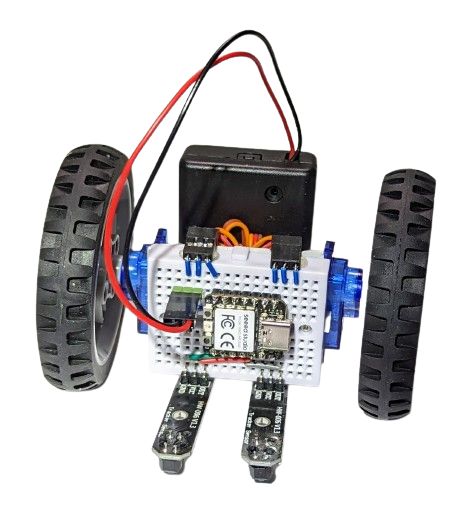
Thanks to the magic of CircuitPython, all it takes now to teach our robot to (even if crudely) follow a line is just three lines of code (boilerplate definitions excluded):

while True:
  servo_left.throttle = 0.1 * line_left.value
  servo_right.throttle = -0.1 * line_right.value

Obstacle avoidance

OK, a line follower implemented with a three-line algorithm is cool, can we do anything else? Sure, look how conveniently the ultrasonic distance sensor fits onto our breadboard:

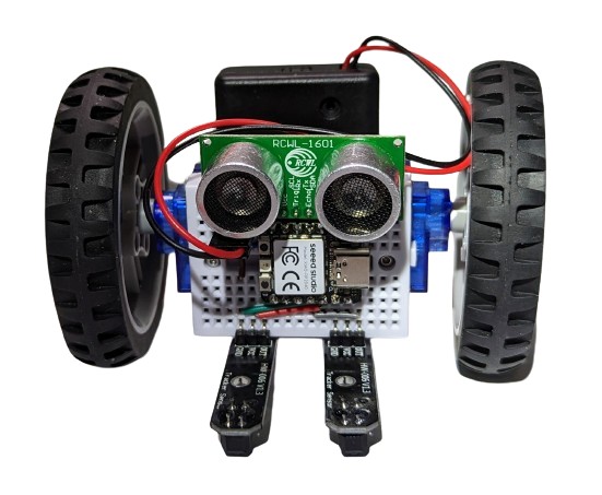
Add a few more lines of uncomplicated Python code and you get a shy robot that can follow a line but will also happily go roaming around your room, steering away from any walls or obstacles:

Note how you can hear the sonar working in the video (not normally audible).

... and more

There is still enough space on the breadboard to add a button and a buzzer:

.. or splash some color with a Xiao RGB matrix:

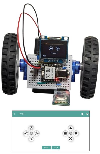
.. or plug in an OLED screen to give your BreadboardBot a funny animated face:
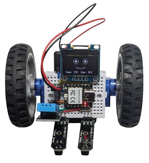
The one on the image above also had the DHT11 sensor plugged into it, so it shows humidity and temperature while it is doing its line following. Why? Because it can!

Tired of programming and just want a remote-controllable toy? Sure, plug in a HC06 bluetooth serial module, program one last time, and go steer the robot yourself with a smartphone:

Other microcontroller boards, BLE, Wifi and FPV

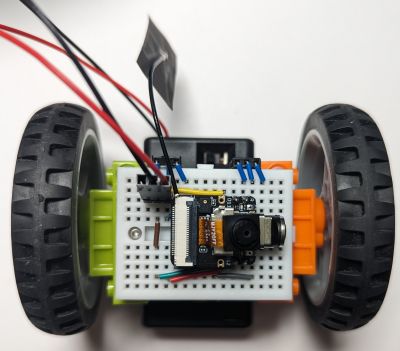
Xiao RP2040 is great, but it has no built-in wireless connectivity! Plug in its ESP32-based cousin Xiao ESP32S3 and you can steer your robot with a Bluetooth gamepad, or via Wifi, by opening a webpage served by the robot itself!
If you have the Xiao ESP32S3 Sense (the version with a microphone and camera), that webpage can even show you the live first-person view feed of the robot's camera (conveniently positioned to look forward):

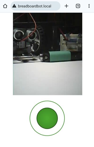
In case you were wondering, the resulting FPV bot is not a very practical solution for spying on your friends, as the microcontroller heats up a lot and consumes the battery way too fast, but it is still a fun toy and an educational project.

Finally, although the Xiao boards fit quite well with all other gadgets on the mini breadboard you are not limited by that choice either and can try plugging in any other appropriately-sized microcontroller board. Here is, for example, a BreadboardBot with an M5Stack Atom Lite running a line-follower program implemented as an ESPHome config (which you can flash over the air!).

Conclusion

The examples above are just the tip of the iceberg. Have any other sensors lying around from those "getting started with Arduino" kits that you did not find sufficiently exciting uses for so far? Maybe plugging them into the BreadboardBot is the chance to shine they were waiting for all this time! Teaching the robot to recognize familiar faces and follow them? Solving a maze? Following voice commands? Self-balancing? Programming coordinated movement of multiple robots? Interfacing the robot with your smart home or one of these fancy AI chatbots? Organizing competitions among multiple BreadboardBots? Vacuuming your desk? The sky (and your free time) is the limit here!

Consider making one and spreading the joy of breadboard robotics!

Detailed build instructions along with wiring diagrams and example code are available on the project's Github page. Contributions are warmly welcome!

Presenting is hard. Although I have had the opportunity to give hundreds of talks and lectures on various topics and occasions by now, preparing every new presentation still takes me a considerable amount of effort. I have had a fair share of positive feedback, though, and have developed a small set of principles which, I believe, are key to preparing (or at least learning to prepare) good presentations. Let me share them with you.

1. Start off without slides

Plan your talk as if you had to give it using only a blackboard. Think about what to say and how to say it so that the listener would be interested to look at you and listen to you. You will then discover moments in your speech, where you need to write or draw something on the blackboard. These will be your slides. Remember, that your slides are only there to enhance and illustrate your presentation. Your speech is its main component.

Of course, preparing slides can be a very convenient way to plan your talk, but try not to fall into the popular trap, where your slides end up being the talk, whilst your own role boils down to basically "playing them back" in front of the audience, so that one may start wondering why are you even there.

When you are done with your slides, a useful practice is to go over them and remove all of the text, besides the parts which you would really have to scribble on the blackboard, if the slides were not available. For any piece of text you currently have on the slide, ask yourself, what is its purpose. Usually there are just two possible answers:

1. It is there to help the listener. In this case, what you usually need instead is an illustration. An actual chart, photo or a schematic cartoon, providing the listener with a useful visual aid. Yes, plain text can also be a visual aid sometimes, but it should be your last resort.
2. Alternatively, you put it there only to help yourself - as a reminder of what to speak about next or what specific wording to use. Delete such texts completely and put some effort into memorizing the talk instead. You can make a paper cheatsheet to peek at during the trickier spots. In general, however, if you find it hard to navigate or memorize your talk, perhaps you should have organized it better in the first place. Which leads us to the second rule:

2. Structure around questions

Imagine that you are constrained to explain your point by only asking questions to the audience. The audience would effectively have to present the topic "by themselves" by answering these questions in order. Surprisingly many seemingly complicated topics may be explained in that manner. Of course, you do not need to literally perform the talk by only querying the audience (although I would suggest you try this format at least once - it can be rather fun). The idea is that the imaginary order of questions that need to be asked, is the best order of exposition for your topic. It is this precise order, in which most new statements tend to follow logically from the previous ones not just for you, but also for the audience, who will thus find it easier to track your talk.

3. Presenting is show business

Remember that every presentation is a show. Your goal is not to explain something in the most precise manner, but to do it in the most interesting manner. There is a caveat, of course: the notion of "interestingness" depends on your audience. Presentations made for schoolkids, students, professors and grandmothers differ not because they need to be told different things, but because you need to tell them the same things in different ways. Thus, always tailor your talk to the audience.

One basic rule which fits most audiences, though, is the following: if you may include interactivity in your talk (i.e. if the format and formalities allow for that), do so. The most basic element of interactivity in a typical presentation would be a question to the audience. There are two main kinds of questions:

1. "Leading questions", where you ask the audience to explain the concepts on their own (see part 2 above).
2. "Quiz questions", for checking whether the listener is still on board. This can provide you with real-time feedback and let you know when you need to slow down or speed up.

Smart combination of these two kinds of interactions would nearly always bump the interestingness of your talk up a notch. It is not enough to know what and when to ask, however. The choice of who to direct your questions to is just as important. Try to avoid the widely spread practice of simply throwing questions into the audience "in general" and giving word to whoever jumps up first. This would often engage just the few most extraverted or excited listeners, leaving the rest feeling a bit like outsiders (although semi-anonymous surveys can be fun sometimes). Unfortunately, communicating with the audience is an art which requires a lot of practice and failed attempts to master. While you are not there yet, let me suggest one simple recipe, which I found to be unexpectedly useful for student audiences - the talking pillow game. Pick an object (not necessarily a pillow) and give it to a random listener. That listener now has to answer your next question and pass the object on to their neighbor.

Of course, asking questions is just the most basic way of introducing useful interaction. Some concepts can be explained in the format of an interactive demo. Try devising one, whenever you can. Keep your listeners awake at all costs.

4. Experiment a lot

Remember that every presentation is a chance to try something new. Feel free to experiment with the various styles and formats every time (this is especially true while you are a student and "failing" a yet-another seminar talk is not really a big deal). Try practicing blackboard-only talks. Do a talk where you only ask questions. Try making a talk where you have no text on the slides at all. Make your talk into an interactive workshop. Experiment with the slide types and formats. Try sitting/standing/walking during the talk. Dance and sing (if you're up to). Trying is the only way to figure out what works and what does not work for you.  In any case, carefully rehearse all the elements of your talk which do not yet come naturally. For the first 100 times this would mean rehearsing all of the talk.

5. Film yourself

Always ask someone to film your presentation. Watching yourself is the only way to discover that you are holding your hands strangely, not looking into the audience, swinging back and forth, closing your eyes, and so on. Watching yourself is often a painfully embarrassing, but a pretty much mandatory procedure, if you want to get better.

By popular suggestion this text was cross-posted to Medium.

Suppose you are starting a new data science project (which could either be a short analysis of one dataset, or a complex multi-year collaboration). How should your organize your workflow? Where do you put your data and code? What tools do you use and why? In general, what should you think about before diving head first into your data? In the software engineering industry such questions have some commonly known answers. Although every software company might have its unique traits and quirks, the core processes in most of them are based on the same established principles, practices and tools. These principles are described in textbooks and taught in universities.

Data science is a less mature industry, and things are different. Although you can find a variety of template projects, articles, blogposts, discussions, or specialized platforms (open-source [1,2,3,4,5,6,7,8,9,10], commercial [11,12,13,14,15,16,17] and in-house [18,19,20]) to help you organize various parts of your workflow, there is no textbook yet to provide universally accepted answers. Every data scientist eventually develops their personal preferences, mostly learned from experience and mistakes. I am no exception. Over time I have developed my understanding of what is a typical "data science project", how it should be structured, what tools to use, and what should be taken into account. I would like to share my vision in this post.

The workflow

Although data science projects can range widely in terms of their aims, scale, and technologies used, at a certain level of abstraction most of them could be implemented as the following workflow:

Colored boxes denote the key processes while icons are the respective inputs and outputs. Depending on the project, the focus may be on one process or another. Some of them may be rather complex while others trivial or missing. For example, scientific data analysis projects would often lack the "Deployment" and "Monitoring" components. Let us now consider each step one by one.

Source data access

Whether you are working on the human genome or playing with iris.csv, you typically have some notion of "raw source data" you start your project with. It may be a directory of *.csv files, a table in an SQL server or a HDFS cluster. The data may be fixed, constantly changing, automatically generated or streamed. It could be stored locally or in the cloud. In any case, your first step is to define access to the source data. Here are some examples of how this may look like:

• Your source data is provided as a set of *.csv files. You follow the cookiecutter-data-science approach, make a data/raw subdirectory in your project's root folder, and put all the files there. You create the docs/data.rst file, where you describe the meaning of your source data. (Note: Cookiecutter-DataScience template actually recommends references/ as the place for data dictionaries, while I pesonally prefer docs. Not that it matters much).
• Your source data is provided as a set of *.csv files. You set up an SQL server, create a schema named raw and import all your CSV files as separate tables. You create the docs/data.rst file, where you describe the meaning of your source data as well as the location and access procedures for the SQL server.
• Your source data is a messy collection of genome sequence files, patient records, Excel files and Word documents, which may later grow in unpredicted ways. In addition, you know that you will need to query several external websites to receive extra information. You create an SQL database server in the cloud and import most of the tables from Excel files there. You create the data/raw directory in your project, put all the huge genome sequence files into the dna subdirectory. Some of the Excel files were too dirty to be imported into a database table, so you store them in data/raw/unprocessed directory along with the Word files. You create an Amazon S3 bucket and push your whole data/raw directory there using DVC. You create a Python package for querying the external websites. You create the docs/data.rst file, where you specify the location of the SQL server, the S3 bucket, the external websites, describe how to use DVC to download the data from S3 and the Python package to query the websites. You also describe, to the best of your understanding, the meaning and contents of all the Excel and Word files as well as the procedures to be taken when new data is added.
• Your source data consists of constantly updated website logs. You set up the ELK stack and configure the website to stream all the new logs there. You create docs/data.rst, where you describe the contents of the log records as well as the information needed to access and configure the ELK stack.
• Your source data consists of 100'000 colored images of size 128x128. You put all the images together into a single tensor of size 100'000 x 128 x 128 x 3 and save it in an HDF5 file images.h5. You create a Quilt data package and push it to your private Quilt repository. You create the docs/data.rst file, where you describe that in order to use the data it must first be pulled into the workspace via quilt install mypkg/images and then imported in code via from quilt.data.mypkg import images.
• Your source data is a simulated dataset. You implement the dataset generation as a Python class and document its use in a README.txt file.

In general, remember the following rules of thumb when setting up the source data:

1. Whenever you can meaningfully store your source data in a conveniently queryable/indexable form (an SQL database, the ELK stack, an HDF5 file or a raster database), you should do it. Even if your source data is a single csv and you are reluctant to set up a server, do yourself a favor and import it into an SQLite file, for example. If your data is nice and clean, it can be as simple as:

   import sqlalchemy as sa
   import pandas as pd
   e = sa.create_engine("sqlite:///raw_data.sqlite")
   pd.read_csv("raw_data.csv").to_sql("raw_data", e)

2. If you work in a team, make sure the data is easy to share. Use an NFS partition, an S3 bucket, a Git-LFS repository, a Quilt package, etc.
3. Make sure your source data is always read-only and you have a backup copy.
4. Take your time to document the meaning of all of your data as well as its location and access procedures.
5. In general, take this step very seriously. Any mistake you make here, be it an invalid source file, a misunderstood feature name, or a misconfigured server may waste you a lot of time and effort down the road.

Data processing

The aim of the data processing step is to turn the source data into a "clean" form, suitable for use in the following modeling stage. This "clean" form is, in most cases, a table of features, hence the gist of "data processing" often boils down to various forms of feature engineering. The core requirements here are to ensure that the feature engineering logic is maintainable, the target datasets are reproducible and, sometimes, that the whole pipeline is traceable to the source representations (otherwise you would not be able to deploy the model). All these requirements can be satisfied, if the processing is organized in an explicitly described computation graph. There are different possibilities for implementing this graph, however. Here are some examples:

• You follow the cookiecutter-data-science route and use Makefiles to describe the computation graph. Each step is implemented in a script, which takes some data file as input and produces a new data file as output, which you store in the data/interim or data/processed subdirectories of your project. You enjoy easy parallel computation via make -j <njobs>.
• You rely on DVC rather than Makefiles to describe and execute the computation graph. The overall procedure is largely similar to the solution above, but you get some extra convenience features, such as easy sharing of the resulting files.
• You use Luigi, Airflow or any other dedicated workflow management system instead of Makefiles to describe and execute the computation graph. Among other things this would typically let you observe the progress of your computations on a fancy web-based dashboard, integrate with a computing cluster's job queue, or provide some other tool-specific benefits.
• All of your source data is stored in an SQL database as a set of tables. You implement all of the feature extraction logic in terms of SQL views. In addition, you use SQL views to describe the samples of objects. You can then use these feature- and sample-views to create the final modeling datasets using auto-generated queries like

  select
     s.Key
     v1.AverageTimeSpent,
     v1.NumberOfClicks,
     v2.Country
     v3.Purchase as Target
  from vw_TrainSample s
  left join vw_BehaviourFeatures v1 on v1.Key = s.Key
  left join vw_ProfileFeatures v2 on v2.Key = s.Key
  left join vw_TargetFeatures v3 on v3.Key = s.Key

  This particular approach is extremely versatile, so let me expand on it a bit. Firstly, it lets you keep track of all the currently defined features easily without having to store them in huge data tables - the feature definitions are only kept as code until you actually query them. Secondly, the deployment of models to production becomes rather straightforward - assuming the live database uses the same schema, you only need to copy the respective views. Moreover, you may even compile all the feature definitions into a single query along with the final model prediction computation using a sequence of CTE statements:

  with _BehaviourFeatures as (
   ... inline the view definition ...
  ),
  _ProfileFeatures as (
   ... inline the view definition ...
  ),
  _ModelInputs as (
   ... concatenate the feature columns ...
  )
  select
       Key,
       1/(1.0 + exp(-1.2 + 2.1*Feature1 - 0.2*Feature3)) as Prob
  from _ModelInputs

  This technique has been implemented in one in-house data science workbench tool of my design (not publicly available so far, unfortunately) and provides a very streamlined workflow.

  

  Example of an SQL-based feature engineering pipeline

No matter which way you choose, keep these points in mind:

1. Always organize the processing in the form of a computation graph and keep reproducibility in mind.
2. This is the place where you have to think about the compute infrastructure you may need. Do you plan to run long computations? Do you need to parallelize or rent a cluster? Would you benefit from a job queue with a management UI for tracking task execution?
3. If you plan to deploy the models into production later on, make sure your system will support this use case out of the box. For example, if you are developing a model to be included in a Java Android app, yet you prefer to do your data science in Python, one possibility for avoiding a lot of hassle down the road would be to express all of your data processing in a specially designed DSL rather than free-from Python. This DSL may then be translated into Java or an intermediate format like PMML.
4. Consider storing some metadata about your designed features or interim computations. This does not have to be complicated - you can save each feature column to a separate file, for example, or use Python function annotations to annotate each feature-generating function with a list of its outputs. If your project is long and involves several people designing features, having such a registry may end up quite useful.

Modeling

Once you have done cleaning your data, selecting appropriate samples and engineering useful features, you enter the realm of modeling. In some projects all of the modeling boils down to a single m.fit(X,y) command or a click of a button. In others it may involve weeks of iterations and experiments. Often you would start with modeling way back in the "feature engineering" stage, when you decide that outputs of one model make for great features themselves, so the actual boundary between this step and the previous one is vague. Both steps should be reproducible and must make part of your computation graph. Both revolve around computing, sometimes involving job queues or clusters. None the less, it still makes sense to consider the modeling step separately, because it tends to have a special need: experiment management. As before, let me explain what I mean by example.

• You are training models for classifying Irises in the iris.csv dataset. You need to try out ten or so standard sklearn models, applying each with a number of different parameter values and testing different subsets of your handcrafted features. You do not have a proper computation graph or computing infrastructure set up - you just work in a single Jupyter notebook. You make sure, however, that the results of all training runs are saved in separate pickle files, which you can later analyze to select the best model.
• You are designing a neural-network-based model for image classification. You use ModelDB (or an alternative experiment management tool, such as TensorBoard, Sacred, FGLab, Hyperdash, FloydHub, Comet.ML, DatMo, MLFlow, ...) to record the learning curves and the results of all the experiments in order to choose the best one later on.
• You implement your whole pipeline using Makefiles (or DVC, or a workflow engine). Model training is just one of the steps in the computation graph, which outputs a model-<id>.pkl file, appends the model final AUC score to a CSV file and creates a model-<id>.html report, with a bunch of useful model performance charts for later evaluation.
• This is how experiment management / model versioning looks in the UI of the custom workbench mentioned above:
  

  Experiment management

The takeaway message: decide on how you plan to manage fitting multiple models with different hyperparameters and then selecting the best result. You do not have to rely on complex tools - sometimes even a manually updated Excel sheet works well, when used consistently. If you plan lengthy neural network trainings, however, do consider using a web-based dashboard. All the cool kids do it.

Model deployment

Unless your project is purely exploratory, chances are you will need to deploy your final model to production. Depending on the circumstances this can turn out to be a rather painful step, but careful planning will alleviate the pain. Here are some examples:

• Your modeling pipeline spits out a pickle file with the trained model. All of your data access and feature engineering code was implemented as a set of Python functions. You need to deploy your model into a Python application. You create a Python package which includes the necessary function and the model pickle file as a file resource inside. You remember to test your code. The deployment procedure is a simple package installation followed by a run of integration tests.
• Your pipeline spits out a pickle file with the trained model. To deploy the model you create a REST service using Flask, package it as a docker container and serve via your company's Kubernetes cloud. Alternatively, you upload the saved model to an S3 bucket and serve it via Amazon Lambda. You make sure your deployment is tested.
• Your training pipeline produces a TensorFlow model. You use Tensorflow Serving (or any of the alternatives) to serve it as a REST service. You do not forget to create tests and run them every time you update the model.
• Your pipeline produces a PMML file. Your Java application can read it using the JPMML library. You make sure that your PMML exporter includes model validation tests in the PMML file.
• Your pipeline saves the model and the description of the preprocessing steps in a custom JSON format. To deploy it into your C# application you have developed a dedicated component which knows how to load and execute these JSON-encoded models. You make sure you have 100% test coverage of your model export code in Python, the model import code in C# and predictions of each new model you deploy.
• Your pipeline compiles the model into an SQL query using SKompiler. You hard-code this query into your application. You remember about testing.
• You train your models via a paid service, which also offers a way to publish them as REST (e.g. Azure ML Studio, YHat ScienceOps). You pay a lot of money, but you still test the deployment.

Summarizing this:

1. There are many ways how a model can be deployed. Make sure you understand your circumstances and plan ahead. Will you need to deploy the model into a codebase written in a different language than the one you use to train it? If you decide to serve it via REST, what load does the service expect, should it be capable of predicting in batches? If you plan to buy a service, estimate how much it will cost you. If you decide to use PMML, make sure it can support your expected preprocessing logic and that fancy Random Forest implementation you plan to use. If you used third party data sources during training, think whether you will need to integrate with them in production and how will you encode this access information in the model exported from your pipeline.
2. As soon as you deploy your model to production, it turns from an artefact of data science to actual code, and should therefore be subject to all the requirements of application code. This means testing. Ideally, your deployment pipeline should produce both the model package for deployment as well as everything needed to test this model (e.g. sample data). It is not uncommon for the model to stop working correctly after being transferred from its birthplace to a production environment. It may be be a bug in the export code, a mismatch in the version of pickle, a wrong input conversion in the REST call. Unless you explicitly test the predictions of the deployed model for correctness, you risk running an invalid model without even knowing it. Everything would look fine, as it will keep predicting some values, just the wrong ones.

Model monitoring

Your data science project does not end when you deploy the model to production. The heat is still on. Maybe the distribution of inputs in your training set differs from the real life. Maybe this distribution drifts slowly and the model needs to be retrained or recalibrated. Maybe the system does not work as you expected it to. Maybe you are into A-B testing. In any case you should set up the infrastructure to continuously collect data about model performance and monitor it. This typically means setting up a visualization dashboard, hence the primary example would be the following:

• For every request to your model you save the inputs and the model's outputs to logstash or a database table (making sure you stay GDPR-compliant somehow). You set up Metabase (or Tableau, MyDBR, Grafana, etc) and create reports which visualize the performance and calibration metrics of your model.

Exploration and reporting

Throughout the life of the data science project you will constantly have to sidestep from the main modeling pipeline in order to explore the data, try out various hypotheses, produce charts or reports. These tasks differ from the main pipeline in two important aspects.

Firstly, most of them do not have to be reproducible. That is, you do not absolutely need to include them in the computation graph as you would with your data preprocessing and model fitting logic. You should always try to stick to reproducibility, of course - it is great when you have all the code to regenerate a given report from raw data, but there would still be many cases where this hassle is unnecessary. Sometimes making some plots manually in Jupyter and pasting them into a Powerpoint presentation serves the purpose just fine, no need to overengineer.

The second, actually problematic particularity of these "Exploration" tasks is that they tend to be somewhat disorganized and unpredictable. One day you might need to analyze a curious outlier in the performance monitoring logs. Next day you want to test a new algorithm, etc. If you do not decide on a suitable folder structure, soon your project directory will be filled with notebooks with weird names, and no one in the team would understand what is what. Over the years I have only found one more or less working solution to this problem: ordering subprojects by date. Namely:

• You create a projects directory in your project folder. You agree that each "exploratory" project must create a folder named projects/YYYY-MM-DD - Subproject title, where YYYY-MM-DD is the date when the subproject was initiated. After a year of work your projects folder looks as follows:

  ./2017-01-19 - Training prototype/
                  (README, unsorted files)
  ./2017-01-25 - Planning slides/
                  (README, slides, images, notebook)
  ./2017-02-03 - LTV estimates/
                   README
                   tasks/
                     (another set of 
                      date-ordered subfolders)
  ./2017-02-10 - Cleanup script/
                   README
                   script.py
  ./... 50 folders more ...
  

  Note that you are free to organize the internals of each subproject as you deem necessary.  In particular, it may even be a "data science project" in itself, with its own raw/processed data subfolders, its own Makefile-based computation graph, as well as own subprojects (which I would tend to name tasks in this case). In any case, always document each subproject (have a README file at the very least). Sometimes it helps to also have a root projects/README.txt file, which briefly lists the meaning of each subproject directory.

  Eventually you may discover that the project list becomes too long, and decide to reorganize the projects directory. You compress some of them and move to an archive folder. You regroup some related projects and move them to the tasks subdirectory of some parent project.

Exploration tasks come in two flavors. Some tasks are truly one-shot analyses, which can be solved using a Jupyter notebook that will never be executed again. Others aim to produce reusable code (not to be confused with reproducible outputs). I find it important to establish some conventions for how the reusable code should be kept. For example, the convention may be to have a file named script.py in the subproject's root which outputs an argparse-based help message when executed. Or you may decide to require providing a run function, configured as a Celery task, so it can easily be submitted to the job queue. Or it could be something else - anything is fine, as long as it is consistent.

The service checklist

There is an other, orthogonal perspective on the data science workflow, which I find useful. Namely, rather than speaking about it in terms of a pipeline of processes, we may instead discuss the key services that data science projects typically rely upon. This way you may describe your particular (or desired) setup by specifying how exactly should each of the following 9 key services be provided:

Data science services

1. File storage. Your project must have a home. Often this home must be shared by the team. Is it a folder on a network drive? Is it a working folder of a Git repository? How do you organize its contents?
2. Data services. How do you store and access your data? "Data" here includes your source data, intermediate results, access to third-party datasets, metadata, models and reports - essentially everything which is read by or written by a computer. Yes, keeping a bunch of HDF5 files is also an example of a "data service".
3. Versioning. Code, data, models, reports and documentation - everything should be kept under some form of version control. Git for code? Quilt for data? DVC for models? Dropbox for reports? Wiki for documentation? Once we're at it, do not forget to set up regular back ups for everything.
4. Metadata and documentation. How do you document your project or subprojects? Do you maintain any machine-readable metadata about your features, scripts, datasets or models?
5. Interactive computing. Interactive computing is how most of the hard work is done in data science. Do you use JupyterLab, RStudio, ROOT, Octave or Matlab? Do you set up a cluster for interactive parallel computing (e.g. ipyparallel or dask)?
6. Job queue & scheduler. How do you run your code? Do you use a job processing queue? Do you have the capability (or the need) to schedule regular maintenance tasks?
7. Computation graph. How do you describe the computation graph and establish reproducibility? Makefiles? DVC? Airflow?
8. Experiment manager. How do you collect, view and analyze model training progress and results? ModelDB? Hyperdash? FloydHub?
9. Monitoring dashboard. How do you collect and track the performance of the model in production? Metabase? Tableau? PowerBI? Grafana?

The tools

To conclude and summarize the exposition, here is a small spreadsheet, listing the tools mentioned in this post (as well as some extra ones I added or will add later on), categorizing them according to which stages of the data science workflow (in the terms defined in this post) they aim to support. Disclaimer - I did try out most, but not all of them. In particular, my understanding of the capabilities of the non-free solutions in the list is so far only based on their online demos or descriptions on the site.

I had to replace my SIM card today. The old one was mini-sized and I needed a micro-sized one. My previous SIM card stayed with me for about 20 years or so. I have gone through high school, university, and traveled around to countless places with it. I changed my phone several times, starting from an older, bulkier Nokia through several candy-bar Nokias and a couple of smartphones. My personal computer evolved from a 200MHz Pentium with 16MB RAM to a 2.8GHz quad-core with 32GB RAM. But my SIM card always stayed the same. Let me dedicate this post to the memory of this glorious tiny computer - the most long-lasting and reliable piece of computing equipment I have ever used.

My retiring SIM card. The mobile operator changed its name from Radiolinja to Elisa in 2000, but the SIM card did not care.

What is a SIM card?

Your SIM card is just another smart card, technologically similar to any of the "chip-and-pin" bank cards in your wallet, your ID card and even your contactless public transport tickets (which communicate using the same set of protocols, just wirelessly). Note, however, that banks started to switch from magnetic to "chip-and-pin" credit cards and countries began issuing smart-card-based identity documents only about 15 years ago or so. SIM cards, on the other hand, had been in wide use much earlier, long before the term "smart card" became a popularized buzzword.

All smart cards are built to serve one primary purpose - identification. The card stores a secret key (which is impossible to retrieve without disassembling the card using ultra-high-tech lab equipment), and provides a way to execute the following challenge-response protocol: you send a random string (a challenge) to the card. The card encrypts the string using the stored key and returns the response. The correctness of this response can now be verified by a second party (e.g. the mobile operator, the bank or a website using ID-card authentication). The actual details of the computation differ among the various smart cards. For example, some use symmetric while other - asymmetric cryptography. Some cards provide additional services, such as creating digital signatures or storing information on the card. None the less, identification is always the core function. This explains the name of the SIM card: Subscriber Identity Module. It is a module, which identifies you (the subscriber) to the network provider.

What is inside a SIM card?

The best way to understand what is inside a SIM (or any other type of smart-) card is to connect it to your computer and "talk" to it. Many laptops have integrated smart-card readers nowadays, so if you find a suitable frame for your nano/micro/mini-SIM, you may simply put it into the reader just as you would do with an ID or a bank card.

Old mini-SIM in a frame from a newer card

Note, though, that if your frame is flimsy and not fitting perfectly (as is mine on the photo above) you run the risk of losing the chip somewhere in the depths of the card reader slot before you even manage to slide it in completely. Hence, in my case, a tiny cross-style USB card reader was a more convenient and reliable option:

SIM in a frame in a reader

Plug it in, wait until the system recognizes the device, and we are ready to talk. There are many tools for "talking" to the card on a low level, but one of the best for the purposes of educational exploration is, in my opinion, the program called CardPeek. Let us fire it up. At start up it asks for the card reader to use (note that you can use it to explore both contact and contactless cards, if you have the necessary reader):

Select reader screen

We can now click "Analyzer → GSM SIM", provide the PIN, wait a bit, and have the program extract a wealth of information stored on the card:

SIM card analyzed

Fun, right? Let us now see where all this data came from and what it actually means.

How does it work?

At the hardware level, a smart card has a very simple connector with six active pins, which are designed for sending and receiving data to and from the card:

Smart card connectors (source)

Four pins (VCC, GND, CLK, I/O) are used for the basic half-duplex synchronous serial communication. RST is the reset pin, and VPP is used for supplying the higher voltage when (re)programming the card. When you first connect to the card, the protocol requires to zero the "reset" pin, to which the card will reply by sending a fixed sequence of bytes, identifying the card and its capabilities. It is known as the card's ATR ("Answer To Reset") string. You can see this string listed as the "cold ATR" entry in the screenshot named "SIM card analyzed" above.

Besides providing pre-packaged analysis scripts for various kinds of smart cards, CardPeek allows to send custom commands to the card by using its Lua scripting interface directly. This is what the "Command" text input at the bottom of the screen is for. Let us now switch to the "logs" tab and try sending some commands. First of all, we need to establish the connection to the card. This is done via the card.connect() call:

card.connect() example

The ATR string is received by the reader when the connection is first established. We can obtain it via card.last_atr() and print out to the log window in hex-encoded form using log.print and bytes:format (the documentation for all these APIs is available here):

ATR example

As we see, the ATR for my card happens to be 3BBA9400401447473352533731365320 (in hex).  If you search the web, you will find that this particular ATR is known to be  a signature of the Elisa SIM cards. It is not a random string, though, and every byte has a meaning. In particular:

• 3B is the "initial byte", and this particular value identifies the smart card as a SIM card.
• BA is the "format" byte. Its first four bits (1011) tell us that we have to expect fields TA1, TB1 and TD1 to follow. The last four bits denote the number 10 - the number of "historical bytes" at the end of the ATR.
• 94 is the field TA1, specifying the clock rate of the serial protocol
• 00 is the field TB1, specifying the programming voltage (apparently, the card is not re-programmable)
• 40 tells us that we have to read out another byte field TC2 (this is in the left-side part of the byte, 4 ) and that the card uses T=0 protocol (this is in the right-side part, 0).
• 14 is the promised TC2 field (not sure what it is meant for),
• the last 10 bytes are the "historical bytes", providing card manufacturer-specific information.

Greeting your Card

Now that we are connected, we can send various commands to the card. Let us proceed by example. The first command we might want to send is "VERIFY CHV", which is essentially greeting the card by providing our PIN1 code ("CHV" stands for "Card Holder Verification").

VERIFY CHV (source)

Every smart card command starts with a two-byte identifier (for example, A0 20 is the (hex) identifier of the VERIFY CHV command). It is followed by two parameter bytes P1 and P2. For example, the parameter P1 for VERIFY CHV is always 0, and P2 must indicate the number of the PIN we are submitting (i.e. 1 for PIN1, 2 for PIN2). Next comes P3 - a byte, specifying the length of the data which follows. For VERIFY CHV the data is the provided PIN itself, and it is always 8 bytes long. If the PIN is shorter than 8 bytes, it must be padded by bytes FF. The PIN itself is encoded in plain ASCII (i.e. 1234 would be 31 32 33 34).

Now, supposing my PIN1 is, in fact "1234", I can authenticate myself to the card via CardPeek as follows:

sw, resp = card.send(bytes.new(8, "A0 20 00 01 08 31 32 33 34 FF FF FF FF"))

Here, card.send is the sending command and bytes.new(8, ...) constructs an array of 8-bit bytes from a hex string (see CardPeek reference).

The sw and resp are the two components of the T=0 protocol response. For VERIFY CHV we only care that sw is equal to 9000, which means "OK". Note how this is printed in the log.

VERIFY CHV example

Beware that if you do not receive a 9000 response, it means that the card denied your PIN for some reason. Trying to submit a wrong PIN three times in a row will block the card.

Reading the Data

Now that we have identified ourselves to the card, let us try to read the data stored on it. The data on the card is organized in a hierarchy of files. It is this exact hierarchy that you can observe as the output of the "Analyzer" script. The root file is called "MF", it has the ICCID, TELECOM and GSM sub-files, which, in turn, have a number of predefined sub-files themselves, etc. The names are just conventions, the card itself uses two-byte identifiers for each file. For example, "MF" is actually 3F 00, "TELECOM" is 7F 10, etc. While the card is connected you can navigate around the file structure just like you would do in a normal operating system using the cd command, except that in smart-card lingo the corresponding command is called SELECT.

The binary form of the SELECT command is A0 A4 00 00 02 {x} {y}, where {x} {y} is the file identifier. Just like before, A0 A4 is the command code, 00 00 are the ignored P1 and P2 parameters, and 02 tells us that exactly two bytes must follow.

Consequently, if we wanted to select the file "MF (3f 00)/TELECOM (7F 10)/ADN (6F 3A)", which contains the address book records, we could achieve it by sending the following sequence of commands via CardPeek:

card.send(bytes.new(8, "A0 A4 00 00 02 3F 00"))
card.send(bytes.new(8, "A0 A4 00 00 02 7F 10"))
card.send(bytes.new(8, "A0 A4 00 00 02 6F 3A"))

Selecting files is a common task, and CardPeek provides a convenient shorthand: card.select("#7f10"). For some cards (not mine, unfortunately) it should also be possible to do things like card.select("/7f10/6f3a").

Once we have selected the ADN ("Abbreviated Dialing Numbers") file, we may read out the individual phone numbers from it using the READ RECORD command. The procedure is complicated by the fact that READ RECORD needs to be provided the "record size" as one of its parameters, which, in turn, must be taken from the response data of the last SELECT command, and this must be obtained via the GET RESPONSE command. The complete example would therefore be:

-- Select /TELECOM/ADN
card.select("#7F10")
sw, resp = card.select("#6F3A")

-- Read file metadata
GET_RESPONSE = "A0 C0 00 00"
sw, resp = card.send(bytes.new(8, GET_RESPONSE, bit.AND(sw, 0xff)))

-- Read out first record in the file
sw, resp = card.read_record('.', 1, resp:get(14))

-- Print the record to the log
log.print(log.INFO, resp:format("%P"))

Reading out a phone record

Note that instead of printing the output to the log via log.print you could also show a message box:

ui.readline(resp:format("%P"))

or append a new node to the tree in the "card view" tab:

nodes.append(nodes.root(), {classname="block", 
                            label="Name", 
                            val=resp:format("%P"), 
                            size=#resp})

In fact, at this point you should go and read the script $HOME/.cardpeek/scripts/gsm (beta).lua. It contains the code we ran in the beginning of this post to analyze the card. The script simply sends the relevant commands to the card and appends all responses as nodes to the tree.

Authentication

While data storage is a useful capability of a SIM card, its main purpose is subscriber authentication. Thus, our acquaintance with the SIM card would be incomplete without checking the corresponding function out as well. It is quite simple:

RUN GSM ALGORITHM (source)

That is, the process is the following: we send the byte sequence A0 88 00 00 10, followed by a 16 byte-long challenge string (which is normally given by the mobile operator when the phone joins the network). The SIM card responds with 12 bytes, of which the first 4 we should send back to the mobile operator for verification, and use the remaining 8 as a cipher key.

Before we can use the RUN GSM ALGORITHM command we need to verify our PIN1 (already done) and SELECT the GSM (7F 20) file:

RUN_GSM_ALGO = "A0 88 00 00 10"
GET_RESPONSE = "A0 C0 00 00"
DF_GSM = "#7F20"

CHALLENGE_STRING = "00 00 00 00 00 00 00 00 00 00 00 00 00 00 00 00"

-- Select GSM file
card.select(DF_GSM)

-- Send the challenge data
sw, resp = card.send(bytes.new(8, RUN_GSM_ALGO, CHALLENGE_STRING))

-- Read 12-byte-long response
sw, RESPONSE_STRING = card.send(bytes.new(8, GET_RESPONSE, 12))
log.print(log.INFO, RESPONSE_STRING:format("%D"))

RUN GSM ALGORITHM example

And that is it. I hope you learned to understand and appreciate your SIM card a bit more today.

Every once in a while I happen to find myself in a public network, where all access besides HTTP and HTTPS is blocked by the firewall. This is extremely inconvenient, as I routinely need to access SSH, VPN or other ports besides HTTP(S). Over time I have developed a reasonably fast and simple way of overcoming the restriction whenever I need it. Let me document it here.

Google Cloud Shell

There are probably hundreds of cloud providers nowadays, each of them trying to outcompete the others by offering better, cheaper, faster, or more diverse set of services. One killer feature of the Google Cloud platform is its cloud shell, which gives you command-line access to a tiny Linux virtual machine directly from their webpage for free:

Once you are logged into Google Cloud platform you may open the shell window via this button

Even if you do not have any serious use for a cloud provider, the cloud shell is one good reason to get an account at the Google Cloud platform. Because whenever I find myself locked out of SSH behind a paranoid firewall, I can still SSH into any of my servers via the cloud shell. This works even when your access is limited to an HTTP proxy server.

Once upon a time there was a great service named koding.com, which also provided free access to a Linux console via HTTP. Unfortunately, they have changed their pricing model since then and do not seem to have any similar free offerings anymore. If you know any alternative services that offer a web-based shell access to a Linux VM for free, do post them in the comments.

OpenVPN via HTTPS

Sometimes SSH access offered by the cloud shell is not enough. For example, I would often need to access the company's VPN server. It runs on port 1194 and in a properly paranoid network this port is, of course, also blocked. The way to sneak through this restriction is the following.

1. Launch a server in the cloud, running an OpenVPN service on port 443 (which corresponds to HTTPS). Even the most paranoid firewalls would typically let HTTPS traffic through, because otherwise they would block most of the web for their users.
2. Connect to that VPN server and tunnel all traffic through it to the outside world.
3. Now we are free to connect anywhere we please. In particular, we may open a VPN tunnel to the company's server from within that "outer" VPN tunnel.
4. At this point I would sometimes SSH into a machine behind the company's VPN and never cease to be amused by the concept of having a SSH tunnel within a VPN tunnel within another VPN tunnel.

Let us now go through all these steps in detail.

Setting up an OpenVPN server

We start by launching a machine in the cloud. You are free to choose any cloud provider here, but as we are using Google's cloud shell already anyway (we are working behind a paranoid firewall already, remember), it makes sense to launch the server from Google's cloud as well. This can be as simple as copy-pasting the following command into the same cloud shell prompt:

gcloud compute instances create openvpn-server --zone=europe-west3-a --machine-type=f1-micro --tags=https-server --image=ubuntu-1604-xenial-v20180405 --image-project=ubuntu-os-cloud --boot-disk-size=10GB --boot-disk-type=pd-standard --boot-disk-device-name=openvpn-server

(obviously, detailed documentation of Google cloud functionality is way beyond the scope of this blog post. All the necessary references and tutorials are rather easy to find, though).  You may play with some of the settings passed to the command above, however the choice of the ubuntu-1604-*** image is important, because the script from the next part was only ever tested on that Linux version. The chosen machine type (f1-micro) is the cheapest and should cost around 5 euros per month (if you keep it open constantly), or a matter of cents, if you only use it for some hours.

Launching a machine in the cloud

Once the machine is up, we SSH into it by typing:

gcloud compute ssh openvpn-server

Here we'll need to install and configure the OpenVPN server. This may be a fairly lengthy process of following step-by-step instructions from, for example, this well-written tutorial. Luckily, I've gone through this already and wrote down all the steps down into a replayable script, which seems to work fine so far with the chosen Linux image. Of course, there's no guarantee it will continue working forever (some rather loose configuration editing is hard-coded there). However, as we have just launched a throwaway virtual server, the worst that can happen is the need to throw that server away if it breaks. (Do not run the script blindly on a machine you care about, though). So let's just download and run it:

curl -s https://gist.githubusercontent.com/konstantint/08ab09202b68e4e3542622e99d21a82e/raw/1a3ee68008d5b565565ebb8c126ae68a8cebe549/ovpn_setup.sh | bash -s

Once completed, the script prints the filename "/home/<username>/client-configs/files/client1.ovpn". This is the name of the file which we need to transfer back to our computer. A clumsy, yet fast and straightforward way is to simply copy-paste its contents from the shell into a local text file:

cat /home/your_username/client-configs/files/client1.ovpn

We then select all the output starting from the first lines of the file

client
dev tun
proto tcp
...

all the way down to

...
-----END OpenVPN Static key V1-----
</tls-auth>

(holding "shift", scrolling and clicking the mouse helps).

We then create a new file (on the local machine), name it client1.ovpn (for example), paste the copied text and save. That's it, we have successfully set up an OpenVPN server running on port 443. Type exit in the cloud shell to log out of the server as we don't need to configure anything there.

Setting up an OpenVPN client

Next we must set up an OpenVPN client on the local computer. I am using a Windows laptop, hence the instructions are Windows-specific, although the logic for Linux or Mac should be rather similar. First, install OpenVPN. The nicest way to do it in Windows is via Chocolatey. Open cmd.exe with administrative privileges and:

1. Install Chocolatey, if you still don't have it (trust me, it's a good piece of software to have):

@"%SystemRoot%\System32\WindowsPowerShell\v1.0\powershell.exe" -NoProfile -InputFormat None -ExecutionPolicy Bypass -Command "iex ((New-Object System.Net.WebClient).DownloadString('https://chocolatey.org/install.ps1'))" && SET "PATH=%PATH%;%ALLUSERSPROFILE%\chocolatey\bin"

2. Now install OpenVPN (if you still don't have it):

choco install -y openvpn

3. Launch OpenVPN GUI (Windows button + type "OpenV" + Enter), right-click on the newly appeared tray icon, select "Import File..." and choose the client1.ovpn file we created:

Import OVPN file

4. Once you've done it, the OpenVPN tray menu will offer you a "Connect" option (or a "client1" submenu with a "Connect" option if you have other connections configured already). Click it, observe the connection dialog, wait until the tray icon becomes green, and congratulations, all your traffic is now tunneled through port 443 of the cloud machine you launched some minutes ago.

Connected

You may verify the effect by googling the words "my ip". You are now also free to connect to any ports or services you need.

Tunnel in a Tunnel

As I mentioned in the beginning, having freed myself from the firewalls of a paranoid network administrator, I would then sometimes need to connect to a corporate or a university VPN. This happens to be surprisingly easy (this part is, however, Windows specific - I am not sure how an equivalent action should look like on Linux or Mac, although I'm sure it should be possible).

1. OpenVPN uses a virtual network tunnel adapter to forward traffic. Initially it only installs one such adapter, but if you want to run a tunnel within a tunnel you will need to add a second one. This is done by simply running C:\Program Files\TAP-Windows\bin\addtap.bat with administrator privileges. It only needs to be done once, of course (unless you need to run a tunnel within a tunnel within a tunnel - then you need to add a a third TAP adapter by running addtap.bat again).
2. Now running a VPN within a VPN is simply a matter of asking OpenVPN to "Connect" to VPNs in the appropriate order. As we are already connected to client1, we simply connect to another profile without disconnecting the first one - this will happily forward a tunnel through an existing tunnel. Fun, right?

VPN via VPN

Cleaning Up

If you only needed the VPN temporarily, do not forget to destroy the cloud machine before going home - otherwise you'll have to pay the unnecessary costs of keeping a server up. Destroying servers is simple. Just go back to the cloud shell where we launched the server and run:

gcloud compute instances delete openvpn-server

That's it. You are back at the mercy of the firewalls.

It is not uncommon when a long-running scientific study or an experiment produces results which are, at best, uninteresting. The measured effect may be too weak to be reported on convincingly given the data at hand. None the less, resources have been put into it, many man-months have been spent, and thus a paper must be published. The researcher must therefore present his results in a way convincing enough for the reviewers to be lulled into acceptance.

The following are the three best methods for doing that (and I have seen those being used in practice). Next time you read someone's paper (or write your own), keep them in mind.

1. Use an irrelevant (and preferably strict) hypothesis test.
   Suppose you want to show that a set of measurements in one group differs from the set of measurements in the other group. The typical approach here is the T-test or the Wilcoxon test, both of which detect whether elements in one group are on average greater than those in the other group. If, however, you find that the tests fail on your data (i.e., there is no easily detectable difference in measurement magnitudes), why don't you try something like the Kolmogorov-Smirnov test, which checks whether the distributions of the two groups are different. It is a much stricter condition. In fact the tiniest outlier in your data will easily get you a low p-value and thus something to stick in the face of a reviewer. If even the KS test did not work, try testing something even less relevant, such as, whether your data is normally distributed. Most probably it is not, here's your low p-value! Remember - the smaller your p-values, the better is your paper!
2. Avoid significance testing completely
   If you can't get a low p-value anywhere, do not worry. Significance testing is going somewhat out of fashion nowadays anyway, so it is possible to avoid it and still sound convincing. If one group of measurements has 40% of successes and the other has 42% - why not simply present those two numbers as obvious proof that the second group is better. Using ratios is also a smart idea. Say, some baseline algorithm has a 1% chance of success. You now test your algorithm and discover that out of 10 trials it had 1 success. That means your algorithm has just demonstrated a 10% success rate, which is ten times better than the baseline! Finally, ROC curves can often be used to hide the fact that your data is too tiny to make any conclusions. No one really ever checks for significance of those.
3. Sweep multiple testing under the carpet
   If you are analyzing a dataset with 1000 attributes and 50 datapoints, it is not really very surprising if one of those attributes will seem "interesting" (e.g. highly correlated with the target effect) purely by chance - there is often nothing significant in finding one out of a thousand. However, if you only mention that one (or perhaps 10-50) of the original attributes, your results will magically become significant and no reviewer will be able to catch your cheating.

There are certainly more, and I'll keep the post updated if I come up with a worthy addition. If you have something to add, please do comment.

I have recently realized that my HP 8440p laptop has a built-in "Qualcomm un2420 Broadband Module" device, also known as a "3G modem". For some reason no drivers were preinstalled for it on my system, and with the SIM card slot concealed behind the battery, it was not something I noticed immediately. Once the drivers were installed, the operating system had no problem recognizing the new "Mobile Broadband Connection" opportunity, and with the SIM card in the slot, I could connect to the Internet via 3G, yay.

Knowing that there is more to mobile communication than Internet access, I was wondering whether I could do anything else, like voice calls or SMS. Unfortunately, my attempts of finding any reasonable software packages, which would open up the power of 3G to me at the click of a button, failed. Instead, however, I discovered that it is actually quite easy to communicate with the modem directly. It turns out you can control your shiny bleeding-edge 3.5G device by sending plain old AT commands to it over a serial port. This is the same protocol that the wired grandpa-modems have been speaking since the 70s and it is fun to see this language was kept along all the way into the wireless century.

Let me show you how it works. Try to follow along — this is kinda fun.

Finding your Modem

If your computer does not have a built-in 3G modem, chances are high your garden variety cellphone does (not to mention smartphones, of course). If it is the case, then:

• Switch on the Bluetooth receiver on your phone (for older Nokias this is usually in the "Settings -> Connectivity -> Bluetooth" menu).
• On your computer, go to "Devices and Printers", click "Add a device", wait until your phone appears on the list, double click it and follow the instructions to establish the connection. (I'm talking about Windows 7 here, but the procedure should be similar for most modern OSs).
• Once the computer recognizes your phone and installs the necessary drivers, it will appear as an icon in the "Devices" window. Double click it to open the "Properties" window, and make sure there is a "Standard Modem over Bluetooth link" function or something similar in the list.
  

  Cellphone Functions

• Double-click that "modem" entry, a new properties window opens. Browse along in it, and find the COM port number that was assigned to the modem.
  

  Bluetooth modem at port COM9

If you do have a 3G modem bundled with your laptop (and you have the drivers installed), open the Device manager ("Control Panel -> Device Manager"), find the modem in the list, double click to open the "Properties" page, and browse to the "Modem" tab to find the COM port number.

Laptop 3G modem in Device Manager

Connecting to the Modem

Next thing - connect to the COM port. In Windows use PuTTY to do it. In Linux use minicom. Don't worry about the settings — the defaults should do.

PuTTY connection dialog

Once the connection starts, you will get a blank screen with nothing but a cursor. Try typing "AT+CGMI" followed by a <RETURN>. Note that, depending on the settings of your device and the terminal program, you might not see your letters being typed. If so, you will have to reconfigure the terminal (enable "local echo"). But for now, just type the command. You should get the name of the manufacturer in response. You can also get the word "ERROR" instead. This means that your modem is ready to talk to you, but it either does not support the "AT+CGMI" command OR requires you to enter the PIN code first. We'll get to it in a second. If you get no response at all, you must have connected to the wrong COM port.

Terminal sessions with a Qualcomm (left) and Nokia (right) 3G modems

You can get more information about the device using the "AT+CGMM", "AT+CGMR", "AT+CGSN" commands. Try those.

Authentication

To do anything useful, you need to authenticate yourself by entering the PIN (if you use your cellphone over bluetooth, you most probably already entered it and no additional authentication is needed). You can check whether you need to enter PIN by using the command "AT+CPIN?" (note the question mark). If the response is "+CPIN: READY", your SIM card is already unlocked. Otherwise the response will probably be "+CPIN: SIM PIN", indicating that a PIN is expected to unlock the card. You enter the pin using the "AT+CPIN=<your pin>" command. Please note, that if you enter incorrect PIN three times, YOUR SIM CARD WILL BE BLOCKED (and you will have to go fetch your PUK code to unblock it), so be careful here.

Entering the PIN

Doing Stuff

Now the fun starts: you can try dialing, sending and receiving messages and do whatever the device lets you do. The (nonexhaustive) list of most interesting commands is available here. Not all of them will be supported by your device, though. For example, I found out that the laptop's 3G modem won't let me dial numbers, whilst this was not a problem for a cellphone connected over bluetooth (try the command "ATD<your number>;" (e.g. "ATD5550010;")). On the other hand, the 3G modem lets me list received messages using the "AT+CMGL" command, while the phone refused to do it.

One useful command to know about is "AT+CUSD", which lets you send USSD messages (those "*1337#" codes) to the mobile service provider. For example, the prepaid SIM card I bought for my computer allows to buy a "daily internet ticket" (unlimited high-speed internet for 12 hours for 1 euro) via the "*135*78#" code. Here's how this can be done via terminal.

Sending an USSD code and receiving an SMS

We first send "AT+CUSD=1,*135*78#" command, which is equivalent to dialing "*135*78#" on the phone. The modem immediately shows us the operator's response ("You will shortly receive an SMS with information..."). We then list new SMS messages using the "AT+CMGL" command. There is one message, which is presented to us in the PDU encoding. A short visit to the online PDU decoder lets us decrypt the message - it simply says that the ticket is activated. Nice.

Sending an SMS

Finally, here's how you can send a "flash" SMS (i.e. the one which does not get saved at the receiver's phone by default and can thus easily confuse people. Try sending one of those at night - good fun). We start with an ATZ to reset the modem, just in case. Then we set message format to "text mode" using the "AT+CMGF=1" command (the alternative default is the "PDU mode", in which we would have to type SMS messages encoded in PDU). Then we set message parameters using the "AT+CSMP" command (the last 16 is responsible for the message being 'flash'). Finally, we start sending the message using the "AT+CMGS=<phone number>" command. We finish typing the message using <Ctrl+Z> and off it goes.

Sending a "Flash" SMS

For more details, refer to this tutorial or the corresponding specifications.

All in all, it should be fairly easy to make a simple end-user interface for operating the 3G modem, it is strange that there is not much free software available which could provide this functionality. If you find one or decide to make one yourself, tell me.

Note: This is again a post for sharing personal computer-taming experiences, that aims to help others who might stumble upon simialr problems. Also note, that this is a guest posting kindly presented by Swen Laur.

We as dumb users are often hurting ourselves through ignorance. One of many such traps is Python install on Mac OS X Leopard. First, for most users a new install is completely unnecessary, since Leopard comes with pre-installed Python. However, as top Google hits kindly suggest to install MacPython, we as ignorant users follow the advice. As a result, there will be two versions of Python in the computer. Now if we install setup-tools and easy_install, spooky things start to happen — packages that are installed through easy_install are suddenly inaccessible and nothing seems to work properly.

The explanation behind this phenomenon is simple though a bit technical. Obviously, after having installed MacPython, we have two distributions of Python in our computer:

• /System/Library/Frameworks/Python.framework/Versions/Current/bin/
• /Library/Frameworks/Python.framework/Versions/Current/bin/

which are accessible from the command line through the links in the directories /usr/bin and /usr/local/bin, respectively. On installation, MacPython modifies .bash_login file so that the new path is

/Library/Frameworks/Python.framework/Versions/Current/bin/;${PATH}
and thus the command line invocation of python is translated to

/Library/Frameworks/Python.framework/Versions/Current/bin/python

which, naturally, corresponds to MacPython.

As a second clue, note that setup-tools and easy_install packages come with Leopard's Python itself. More precisely, the corresponding command line tool is /usr/bin/easy_install. However, if you install setup-tools for your new MacPython, the corresponding binary will be  /usr/local/bin/easy_install. Now note that in the default configuration, /usr/bin goes before /usr/local/bin in the PATH variable. As a direct consequence, each invocation of easy_install puts packages to Apple Python (into the directory /Library/Python/<version>/site-packages, to be precise), and these packages are naturally not accessible by the MacPython, that you normally execute from a shell. MacPython search the packages from the directory

/Library/Frameworks/Python.framework/Versions/<version>/lib/python2.5/site-packages.

As a simple solution, we must change the configuration of easy_install. For that we have to change the configuration  .pydistutils.cfg located at your home directory. There should be the following lines

[install]
install_lib=/Library/Frameworks/Python.framework/Versions/Current/lib/python$py_version_short/site-packages/
install_scripts =/Library/Frameworks/Python.framework/Versions/Current/bin

The first line specifies where all Python modules should be installed and the second line specifies where all executables should be located (this directory is in the first place in the PATH and thus  MacPyton executables are the first to be executed). After that one should reinstall setuptools and easy_install.During the installation of setuptools, the program might comlain. In this case you should silence it by modifying PYTHONPATH. As a result, easy_install is located 

/Library/Frameworks/Python.framework/Versions/Current/bin 

and thus the packages are put into correct directory. As such, we solve the problem with easy_install but are still vulnerable to other easter-eggs coming from the fact that we do not use the Apple distribution of Python. In particular, you cannot do any user-interface related programming, since the corresponding PyObjC module is missing from non-Apple Python distributions.

Another, more complex solution is to remove MacPython cleanly. The latter is not an easy thing to do, since package management of open-source tools is more than unsatisfactory in Mac OS X (in fact, open-source tools are often difficult to install and uninstall under many non-Linux operating systems). The situation is even worse when you have installed some other Apple packages (.mpkg files) to extend basic configuration of MacPython. In the following, we describe how to do a successful uninstall in such cases. This procedure is not for the fainthearted — if you have a time-machine copy of the system state before installing MacPython, then it might be easier to revert to this state.

The key to successful uninstallation procedure is a basic understanding what is a package and how the Installer.app works. First, note that the package is nothing more than a directory (one can expand the contents by right-clicking the package) with the following structure

Contents/Archive.bom
Contents/Info.plist
Contents/Packages/..
Contents/PkgInfo
Contents/Resources

The file Info.plist provides an xml-description how to install the package. The file Archive.bom contains in semi-binary description of all files that will be copied to various install locations. The directories Packages and Resources contain sub-packages and files to be copied to the system. The installer.app reads Info.plist and Archive.bom to create necessary files and then copies the package without directories Resources to /Library/Receipts. The receipts are in principle enough to do a clean uninstall if the files are not used by other programs. Normal practice for the Apple software requires that all files should be stored in the directory
/Applications/Installed-Application.app or in some place in /Library if the corresponding piece of software is shared by several applications. Mostly, the corresponding directories are stored in /Library/Frameworks.  The integrity of all files installed under /System during the system updates are not guaranteed and therefore sane persons do not store files there. The latter is not true for open-source software, which often tries to write into directories /usr/local/bin and /usr/bin (extremely dangerous).

To uninstall packages, we have to first find out, where it was written. The  key IFPkgFlagDefaultLocation or IFPkgRelocatedPath in the Info.plist contains the default or actual installation directory. With the command line tool lsbom we can also see the list of all files and directories that where installed. To be precise, the lsbom gives out relative paths with respect to install directory.

Now applying this knowledge, we can deduce that MacPython consists of five packages, which create a directory /Library/Frameworks/Python.framework
and write the following files

idle
idle2.5
pydoc
pydoc2.5
python
python-config
python2.5
python2.5-config
pythonw
pythonw2.5
smtpd.py
smtpd2.5.py

to the directory /usr/local/bin in addition to /Application/MacPython <>. Hence, if we remove these files, we restore the initial state unless we installed some other packages. In this case the procedure can be more tedious.

Finally, we should restore the old ~/.bash_login from the file ~/.bash_login.pysave.

To summarize, uninstallation of packages is more difficult than application-bundles (yet nevertheless, it is not hopeless). But still, I think applications without installers are the way to go.

Important update: How to install scypy from source code

Scipy is a nice extension of Python that provides the power of Matlab functions. By some odd reasons the maintainers of scipy package suggest to install non-Apple distribution of Python. In other words, they force you to abandon PyObjC library that is a core graphical library on Mac OS X. Fortunately,  it is still possible to have both by installing scipy package from the source. There are some hiccups in the procedure but in general it is doable

1. Install unfpack thogether with UFconfig and AMD libraries from the source
   1. Download source files from the url http://www.cise.ufl.edu/research/sparse/umfpack/
   2. Change the configuration file UFconfig according your computer. Flag
       
      UMFPACK_CONFIG = -DNBLAS  

      is a safe though a bit slow choice 

   3. Run make and pray
   4. Copy libumfpack.a  and libamd.a

   to /usr/local/lib

   5. Copy all files from Include directories of UMPACK, UFconfig and AMD:
      

      umfpack*.h
      UFconfig.h
      amd.h
      amd_internal.h

2. Download and install numpy and scipy packages. You might change the compilation target by by typing the following commandexport MACOSX_DEPLOYMENT_TARGET=10.4in the shell before compiling and installing. The target value 10.5 is not good choice, since it automatically creates compile problems (joys of using freeware). Note that the current tarball scipy-0.7.0b1 is incomplete (joys of using freeware) and thus you have to use svn trunc for that. But otherwise, the installation guide http://www.scipy.org/Installing_SciPy/Mac_OS_X is correct.

Important update: An update to the update

Seems that they have now fixed the 10.5 target and you can use the command

export MACOSX_DEPLOYMENT_TARGET=10.5

before compiling if you have Leopard

Note: This is a brief transcript of actions related to my recent hard disk crash recovery. I'm publishing it here in the hope it might be of use to someone someday, just as all those similar posts out there are every so often of great use to me. So if you, dear reader, are not really interested in replacing a hard disk of your DELL PC, you better save your time and skip to the next post.

A pair of days ago I accidentally managed to test what happens if you throw a running 3-year-old DELL XPS M1210 laptop from a height of about 1.3 meters against solid floor. The result, fortunately, was radically different from what one might expect after observing that painful inelastic crash. After switching the screen off for a period of 5 seconds or so (the reasons behind this behavior being a complete mystery for me) the laptop happily resumed as if nothing had happened. A later examination revealed that the only part that was damaged was the hard disk where a number of files became unreadable.

I presumed that it must have been the result of a strong head crash. Common knowledge suggests that a head-crashed hard disk should better be replaced, even if it continues functioning. This is because new head crashes are much more probable after the first one has happened. Thus, I went to the shop and got myself a new average-grade 160Gb SATA hard disk (these are surprisingly cheap nowadays, btw). I also bought a small external case to put my old drive into, so that I could continue using it as an external storage medium.

In principle, the whole procedure could have ended here: I could have taken the old hard disk out, put the new one in, installed the OS onto the new disk from a CD and copied my files from the old disk with the help of the external case. However, there was one thing I didn't like about this approach. If I were to restart with a blank OS, I'd have to bother installing the proper drivers as well as several pieces of software that were shipped with the factory preinstallation of Windows XP (in particular, that enormously useless yet really impressive Logitech Video Effects webcam feature). I knew, however, that there was a way to restore the disk to the factory setting so I went on to figure out how to do it for a new hard disk. In hindsight, the whole procedure is actually rather straightforward, at least if you appreciate the virtues of the dd command.

DELL System Restore Partition

It seems that most DELL laptops nowadays come with a "DELL System Restore" feature, which means that there is a hidden partition on the hard disk that stores the factory-installed Ghost image of the system drive. If at boot time you press Ctrl+F11, you get the opportunity to write this image to disk thus destroying all your data but bringing the computer to its retail state.

The hidden partition is labeled DellRestore and besides the image file it contains a bootable DOS operating system (yes, real DOS!), the program for restoring the Ghost image (restore.exe) and an autoexec.bat script that invokes this program on boot. So, if I'm not mistaken, by pressing Ctrl+F11 you just direct the laptop to boot the DellRestore partition.

In theory, if you mirror the partition structure of your old hard drive on the new one and copy the data of the DellRestore partition, it should be possible to simply put in the new drive and press Ctrl+F11 for a proper restoration. However, my new drive was larger in capacity than the old one so I didn't want to mirror the partition structure exactly and I ended up with a somewhat more complicated procedure. The following is an approximate list of steps I went through. Don't try repeating them unless you really understand everything, though. You are also strongly advised to visit this site first.

The Walkthrough

1. I needed two bootable CDs here: one Knoppix Live CD and one DOS bootable CD.
2. First, keep the old (damaged) hard disk in the laptop, put the new disk into the external case, but don't plug it in yet.
3. Boot the Knoppix CD, when it starts switch to the command line (Ctrl+Alt+F1)
4. Ensure that the laptop's hard disk is seen as /dev/sda and examine its partition table:
   # cfdisk /dev/sda
5. It should have 3 partitions: DellUtility (sda1), the main NTFS partition (sda2) and DellRestore (sda3). Write down their sizes and quit cfdisk.
6. Plug in the new disk (the one in the external case) into the USB port. Ensure that OS detects it: type
   # dmesg
   and examine the output.
7. 

   New Drive's Partition Table

   Type
   # cfdisk /dev/sdb
   and create a partition table for the new disk that mimics the one of the old one. In my case I created the first DellUtility partition of the same size and type as was sda1. I then added one NTFS partition (for the main Windows OS) and a small Linux partition (just for fun) choosing the sizes of both to my liking. Finally the fourth partition was created of the same size and type as sda3. See Figure.

8. Copy the data of sda1 to sdb1 and sda3 to sdb4.
   # dd if=/dev/sda1 of=/dev/sdb1 bs=1024
# dd if=/dev/sda3 of=/dev/sdb4 bs=1024
9. Copy the master boot record of the old drive to the new one.
   # dd if=/dev/sda of=/dev/sdb bs=446 count=1
10. Now, shutdown Knoppix
    # shutdown -h now
    remove the old disk from the laptop, take the new disk from the case and put it into the laptop. Now boot the DOS CD.
11. When in DOS, go to disk C: (this is the DellRestore partition) subdirectory bat\:
    > cd c:\bat
12. Execute restore.bat
> restore.bat
    This should initiate the restore process and write the factory image to your second partition.
13. After the restore process completed I somewhy still had the problem that the system would not boot. I booted Knoppix, opened the partition table (cfdisk /dev/sda) and discovered that the bootable flag of the second partition was gone after the restoration process. Making the partition bootable again and restarting fixed the problem.

That's it.

I received a number of "why" and "how" questions regarding the pri.ee domain name of this site and I thought the answers are worth a post. The technically savvy audience can safely skip it, though.

The pri.ee subdomain is reserved by EENet for private individuals, who have an estonian ID code. The registration is free of charge and very simple: you just fill in a short form and wait a day or two until your application is processed. As a result you end up with a simple affiliation-free way of designating your site. Of course, it does not have the bling of a www.your-name.com, but I find it quite appropriate for an aspiring blog (and besides, I'm just too greedy and lazy to bother paying for the privilege of a flashy name for my homepage).

Now on to the "how" part. The only potentially tricky issue of the registration process is the need to fill in the "Name servers" field. Why do you need that and why can't you just directly provide the IP address of the server where you host your site? Well, if you could register the specific IP of your server with EENet, you would have to to contact EENet every time your hosting provider changed, right? In addition, you would need to bother EENet about any subdomain (i.e. <whatever>.yourname.pri.ee) you might be willing to add in the future. Certainly not the most convenient option. Therefore, instead of providing an IP address directly, you specify a reference to an intermediate server, which will perform the mapping of your domain name (and any subdomains) to IP addresses. That's how the internet domain naming system actually works.

So which name server should you choose? Most reasonable hosting providers (that is, the ones that allow to host arbitrary domains) allow you to use their name servers for mapping your domain name. The exact server names depend on the provider and you should consult the documentation. For example, if you were hosting your site at 110mb.com (which is here just an arbitrarily chosen example of a reasonable free web hosting I'm aware of), the corresponding name servers would be ns1.110mb.com and ns2.110mb.com.

However, using the name server of your provider is, to my mind, not the best option. In most cases the provider will not allow you to add subdomains and if you change your hosting you'll probably lose access to the name server, too. Thus, a smarter choice would be to manage your domain names yourself using an independent name server. Luckily enough, there are several name servers out there that you can use completely free of charge (or for a symbolic donation): EveryDNS and EditDNS are two examples of such services that I know of.

After you register an account with, say, EveryDNS, you can specify the EveryDNS nameservers (ns1.everydns.net, ..., ns4.everydns.net) in the pri.ee domain registration form. You are now free to configure arbitrary address records for yourname.pri.ee or <whatever>.yourname.pri.ee to your liking.

To summarize, here how one can get a reasonable website with a pri.ee domain name for free:

1. Register with a reasonable web hosting provider
   • 110mb.com is one simple free option (with an exception that they charge $10 once if you need MySQL)
   • other options
2. Register a DNS account
   • EveryDNS
   • other options
3. Fill out this form.
   • If you chose EveryDNS in step 2, state ns1.everydns.net, ns2.everydns.net, ns3.everydns.net, ns4.everydns.net as your name servers.
   • Wait for a day or two.
4. Suppose you applied for yourname.pri.ee (the domain is still free, by the way!), then:
   • Add this domain in your hosting's control panel and upload your website.
   • Add this domain to your DNS account.
     • You can add an A ("address") record mapping yourname.pri.ee to an IP address.
     • Alternatively, you can add a NS ("name server") record referencing yourname.pri.ee further to ns1.110mb.com (or whatever name server your hoster provides).
5. Profit!